
Abstract
China’s 2026 economy combines rapid growth in selected high-technology manufacturing and exports with weak private investment, prolonged property adjustment, subdued household credit, and soft consumer demand. This paper asks how technology-intensive growth reaches households through the labor market and where that transmission can weaken.
The analysis combines a published-benchmark replication with an original China Family Panel Studies extension. First, an independent reimplementation of the public analytical package for Giuntella, Lu, and Wang reproduces all six headline Table 2 2SLS coefficients at the authors’ displayed three-decimal precision. Second, public prefecture robot exposure is aggregated to province using baseline employment weights and linked to CFPS respondents observed between 2012 and 2016. In the baseline-employment province specification, one standard deviation of additional 2010–2014 robot exposure is associated with an approximately 2.5 percentage-point decline in employment. The sign remains negative under an alternative 1982 shifter, after excluding automotive or electronics exposure, under attrition adjustment, and in every leave-one-province-out estimate.
The new employment estimate is deliberately classified as qualified. The public-CFPS extension contains 25 observed province treatment units, and the main external shifter is correlated with baseline age, education, and urbanization. Adding the full baseline composition vector attenuates the equal-weight estimate to about -1.5 percentage points per standard deviation and widens the interval across zero. Survey-weighted individual specifications show the same loss of precision under the main shifter.
Household outcomes do not show a stable collapse in total personal consumption expenditure. Instead, expenditure composition moves more consistently: the all-province estimates imply approximately +2.75 percentage points in food share and -0.97 percentage points in housing share per standard deviation of automation exposure. Mortgage holding also falls in the full sample but is sensitive to municipality exclusion. A later within-person job-security panel associates higher reported security with fewer weekly hours, greater contract coverage, and more insurance in the 2016–2020 window, but those mechanism results weaken in the pre-pandemic window and are not interpreted causally. An earlier apparent security-to-household-income/savings result disappears after duplicate household-year outcomes are removed.
The evidence supports a narrow Growth-to-Wallet conclusion. Technology exposure can generate labor-market displacement while total household expenditure remains smooth, with adjustment appearing in job attributes and spending composition. The paper does not identify historical robot adoption as the cause of China’s weak household demand in 2026. Property adjustment, demographics, fiscal composition, external demand, corporate profitability, and credit conditions remain competing contemporary mechanisms.
Keywords: China; industrial automation; labor markets; household consumption; job security; consumption smoothing; shift-share instruments; K-shaped growth.
Evidence, authorship, and scope
This is an independent Galok empirical research paper. Numerical results are separated by provenance.
Published benchmark. The underlying causal design and author-supplied estimates belong to Giuntella, Lu, and Wang. This paper independently reimplements their public final analytical files and reports the reproduction status explicitly.
Original empirical estimates. Province-level CFPS employment and household-transition results, robustness grids, multiple-testing adjustments, and job-security fixed-effects estimates are generated by the analysis code accompanying this paper. They are reported with the treatment geography and identification limitations stated in Sections 5–10.
Current macro evidence. The 2026 production, finance, labor, and consumption figures motivate external relevance. They are descriptive and dated to their cited releases.
Testable extensions. Employer-power interactions, the Rights-Exercise Penalty, and perceived recoverability remain conceptual or future empirical modules unless direct evidence is reported. They are not presented as established findings.
No restricted CFPS microdata are redistributed. Public replication files contain code, variable dictionaries, aggregate outputs, and figures only.
1. Introduction
1.1 The puzzle
China entered the second half of 2026 with an economic configuration that is difficult to summarize using a single growth rate. In the first seven months of the year, value added among industrial enterprises above designated size rose by 5.3 percent year on year. Equipment manufacturing expanded by 9.7 percent and high-technology manufacturing by 13.8 percent. Output of industrial robots rose by 28.5 percent. Merchandise exports increased by 14.0 percent, while exports of mechanical and electrical products grew by 21.2 percent and accounted for 63.8 percent of total exports. Over the same period, fixed-asset investment fell by 6.7 percent, private investment by 9.4 percent, and real-estate development investment by 19.2 percent. Retail sales of consumer goods increased by only 1.2 percent, with July growth slowing to 0.6 percent. The National Bureau of Statistics (NBS) described the imbalance between strong supply and weak demand as acute (National Bureau of Statistics of China, 2026a).
Credit data reveal a related split. At the end of July 2026, broad money stood at RMB 355.51 trillion, while household deposits had increased by RMB 6.95 trillion during the first seven months. Yet household loans fell by RMB 827.1 billion over the same period. Government-bond financing remained large: net government-bond financing reached RMB 7.76 trillion over January–July, while loans to the real economy grew more slowly than a year earlier (People’s Bank of China, 2026). The combination is important because it separates aggregate financial abundance from private willingness to borrow and spend. A large monetary stock can coexist with defensive household balance sheets.
International institutions describe the same broad tension from a different angle. The World Bank’s July 2026 China Economic Update characterizes early-2026 growth as resilient but increasingly dependent on high-technology investment, policy support, and exports while consumption and the property sector remain weak. It argues that rebalancing toward household consumption is gradual and highlights social protection as one channel through which precautionary saving could be reduced (World Bank, 2026). The IMF’s 2025 Article IV consultation, published in February 2026, similarly identifies prolonged weakness in domestic demand, continued property-sector adjustment, and strong exports that partly absorb domestic slack. The IMF also warns that reliance on exports is less viable as a long-run growth strategy for an economy of China’s size amid greater global trade tensions (International Monetary Fund, 2026).
These observations motivate the central question of this paper:
How does capital- and technology-intensive industrial upgrading in China pass through into employment, labor income, job security, and household consumption, and how is that pass-through altered by employer labor-market power and labor-market institutions?
The key word is pass-through. Industrial output can expand without producing a proportional increase in employment. Productivity gains can be divided differently between firms and workers depending on labor-market structure. Workers who remain employed can face changes in hours, contract security, work intensity, or schedule control that are invisible in a binary employment measure. Household consumption can respond to future income risk even before current income falls. A household can also maintain total expenditure temporarily by borrowing, using liquid savings, receiving transfers, or reallocating spending away from deferrable categories.
The paper therefore treats growth as a sequence rather than a scalar:
\[ Technology/Capital \rightarrow Output/Productivity \rightarrow Employment\;and\;Job\;Quality \rightarrow Labor\;Income \rightarrow Income\;Expectations \rightarrow Household\;Demand. \]
A weak link at any stage can produce a divergence between strong production and weak household demand.
1.2 Why the labor market is the central transmission layer
For households without substantial business ownership or financial portfolios, the most important economic asset is the expected stream of future labor income. Industrial growth reaches such households primarily through work. Employment quantity matters, but so do wages, hours, stability, contract protection, social insurance, and the probability of obtaining another job if the current job disappears.
The aggregate Chinese labor market illustrates why a headline unemployment rate is insufficient. The urban surveyed unemployment rate averaged 5.2 percent in the first seven months of 2026, while enterprise employees worked an average of 48.2 hours per week in July (National Bureau of Statistics of China, 2026a). These figures should not be read as proof of either a healthy or distressed labor market. They show that employment status and labor intensity can move independently. The economic adjustment to a technology or demand shock can occur through hours, task scope, compensation, worker turnover, contract form, or perceived security without appearing fully in unemployment.
Structural transformation adds another layer. New industries can create valuable jobs while generating substantial worker-level transition costs. The World Bank’s 2026 analysis of China’s low-carbon transition emphasizes rising demand for green and transferable skills but also substantial skill mismatch and uneven geographic mobility (World Bank, 2026). A newly created technical position in one region is not an automatic substitute for a displaced worker in another region with different skills, age, family constraints, or housing ties.
Employer power matters at the next stage. Productivity gains do not mechanically become wage gains. Search frictions, commuting costs, occupation-specific human capital, information asymmetries, non-compete restrictions, and a small number of credible alternative employers can give firms wage-setting power. In such settings, two regions can experience similar productivity growth while workers capture different portions of the gain.
Labor institutions can reinforce or mitigate these mechanisms. A formal right has economic value only when workers can use it at tolerable cost. The cost of claiming unpaid wages, challenging excessive working time, or contesting an employment classification includes time, evidence, legal uncertainty, current-employer retaliation, and potentially future employment consequences. Recent Chinese legal developments have clarified several dimensions of labor protection, including non-compete restrictions, mixed employment, platform work, social insurance, and digitally mediated overtime. The existence of those protections does not settle their effective value. That depends on enforcement and worker outside options.
1.3 Why the household response matters for macroeconomic rebalancing
The household side is not only a welfare outcome. It affects the sustainability of growth composition.
When households expect stable future labor income, a discretionary purchase can be treated as a temporary reduction in liquidity. When expected re-employment becomes difficult or wages feel insecure, the same purchase can carry a much higher perceived economic cost. Standard permanent-income and precautionary-saving theories already explain why future income risk matters for present consumption. This paper builds on that foundation rather than competing with it.
The narrower household question is whether labor-income insecurity changes which expenditures are cut first, and whether total consumption can remain deceptively stable because households use debt, savings, or family insurance. If households preserve food, housing, and other difficult-to-defer expenditure while postponing travel, entertainment, durable replacement, or other flexible purchases, aggregate consumption can conceal meaningful stress in consumption composition.
This mechanism can interact with private investment. A stylized feedback is:
\[ Weak\;Job/Income\;Expectations \rightarrow Precautionary\;Saving \rightarrow Weak\;Discretionary\;Demand \rightarrow Weaker\;Private\;Revenue\;Expectations \rightarrow Lower\;Hiring/Investment. \]
The paper does not assume this entire macro feedback is identified. The chain organizes measurable components; broader general-equilibrium effects remain interpretation unless separately identified.
1.4 Contributions
The paper makes four contributions at different evidentiary levels.
First, it passes a replication gate before presenting new results. An independent reimplementation of the Giuntella–Lu–Wang public final analysis files reproduces all six headline Table 2 2SLS coefficients at the authors’ displayed three-decimal precision. This anchors the extension in a published China robot design whose treatment scaling and fixed-effect structure have been independently reconstructed.
Second, it adds a public-CFPS province extension with explicit identification limits. Permanent individual identifiers are used to follow workers from 2012 to 2016, while published prefecture robot exposure is aggregated to province using baseline employment weights. The new estimates show a persistent negative employment direction under alternative shifters, sector exclusions, attrition adjustment, and leave-one-province-out estimation. The paper also documents why the result is qualified: baseline province education, urbanization, and age are correlated with the external shifter, and full baseline controls weaken precision.
Third, it moves the household outcome from a headline total to the composition of spending. The same province extension does not produce a stable directional response in total PCE. Food share rises and housing share falls more consistently. This provides original evidence for a narrower household-adjustment claim: the composition margin can move even when total expenditure is statistically smooth.
Fourth, it subjects its own mechanism results to unit-of-observation and period audits. Worker fixed-effects estimates connect subjective job security to hours, contracts, and insurance in the 2016–2020 panel, with weaker evidence in the pre-pandemic window. An earlier apparent household income/savings relationship disappears when duplicate household-year outcomes are removed. The failed result is retained as part of the evidence rather than hidden.
The broader employer-power, Rights-Exercise Penalty, and recoverability concepts remain testable extensions. They are not needed for the core empirical paper to survive.
The resulting contribution is a calibrated Growth-to-Wallet map:
\[ Industrial\ Upgrading \rightarrow Labor\ Market \rightarrow Household\ Adjustment, \]
with a clear distinction between reproduced causal evidence, qualified original estimates, mechanism associations, and unsupported links.
1.5 Evidence and replication architecture
The paper separates four evidence classes.
- Current descriptive evidence establishes the 2026 macroeconomic puzzle. It is dated and does not identify the historical automation coefficients.
- Published causal evidence comes from the China robot literature and related labor/household research.
- Independent replication evidence reproduces the published robot benchmark coefficients from the authors’ public final analysis files.
- Original Galok estimates use public CFPS and the public province robot-exposure reconstruction. Their causal language is weaker where treatment geography, balance, or inference is weaker.
The empirical hierarchy is therefore fixed before interpretation. A successful benchmark replication cannot make a weak new extension causal. A significant household coefficient cannot rescue an imbalanced instrument. A null total-consumption result cannot be upgraded to perfect consumption smoothing. A mechanism fixed-effects result cannot be described as exogenous simply because person fixed effects are included.
Sections 5 and 6 document the actual data build and estimators. Section 7 retains optional institutional extensions. Section 8 reports original empirical results, Section 9 stress-tests them, Section 10 evaluates mechanisms, Section 11 gives policy interpretation, and Section 12 concludes.
2. Stylized Facts: Four Layers of the K
The K-shaped pattern relevant to this paper appears in several domains at once. The facts below establish the research environment. They do not identify causality. Current Chinese official series are used as high-frequency measurements and are cross-read with international institutional assessments and published microeconomic evidence; they do not carry the paper’s causal claims.
2.1 Production and investment
The first divergence appears in production and capital expenditure.
In January–July 2026, industrial value added rose by 5.3 percent, equipment manufacturing by 9.7 percent, and high-technology manufacturing by 13.8 percent. Production of industrial robots, lithium-ion batteries, and 3D-printing devices grew rapidly. At the same time, total fixed-asset investment fell by 6.7 percent, manufacturing investment by 1.7 percent, real-estate development investment by 19.2 percent, and private investment by 9.4 percent. Private investment excluding real estate still fell by 5.7 percent. Within this weak aggregate, high-technology industry investment increased by 5.0 percent; information-services investment rose 19.2 percent, aerospace vehicle and equipment manufacturing 12.3 percent, and electronic and communication equipment manufacturing 7.1 percent (National Bureau of Statistics of China, 2026a).
The first layer can be summarized as:
\[ Strategic/High\text{-}tech\;Capital\uparrow \]
alongside:
\[ Private/Property/Broad\;Investment\downarrow. \]
This does not imply that strategic investment caused private investment to decline. Property adjustment, profitability, expected demand, local fiscal conditions, financing structure, and external shocks can all generate the same cross-sectional pattern. The stylized fact is that capital formation is highly uneven across sectors.
Exports add a second demand source. Over the same seven months, merchandise exports rose by 14.0 percent and mechanical/electrical exports by 21.2 percent (National Bureau of Statistics of China, 2026a). Selected manufacturing sectors can therefore face strong external demand while domestic consumption and broad private investment remain weak.
Selected January–July 2026 growth rates
DESCRIPTIVE / NBSStatic figure and accessible values follow.
| Indicator | Year-on-year change |
|---|---|
| Goods exports | +14.0% |
| High-tech manufacturing value added | +13.8% |
| Equipment manufacturing value added | +9.7% |
| Industrial value added | +5.3% |
| High-tech industries investment | +5.0% |
| Retail sales of consumer goods | +1.2% |
| Manufacturing investment | −1.7% |
| Fixed-asset investment | −6.7% |
| Private investment | −9.4% |
| Real-estate development investment | −19.2% |
Source: National Bureau of Statistics of China, National Economy Maintained Steady Momentum with Innovation-driven and High-quality Development in the First Seven Months, 17 August 2026. https://www.stats.gov.cn/english/PressRelease/202608/t20260817_1965057.html
2.2 Finance and credit
The second divergence appears in finance.
At end-July 2026, M2 stood at RMB 355.51 trillion, 7.7 percent higher than a year earlier. Household deposits increased by RMB 6.95 trillion during the first seven months. Yet household loans fell by RMB 827.1 billion. Aggregate financing to the real economy still expanded, supported in part by government and corporate bond financing: net government-bond financing reached RMB 7.76 trillion and corporate-bond financing RMB 2.52 trillion over January–July (People’s Bank of China, 2026).
The important distinction is between:
\[ Availability\;of\;Financial\;Resources \]
and:
\[ Private\;Willingness\;to\;Leverage. \]
A household can increase deposits because it values liquidity more highly. A government or strategic borrower can continue financing while households and private firms behave defensively. The second K therefore concerns financing composition, not a claim that the economy lacks money.
Selected January–July 2026 financing and balance-sheet changes
DESCRIPTIVE / PBCStatic figure and accessible values follow.
| Flow / balance-sheet change | RMB trillion |
|---|---|
| Loans to enterprises and public institutions | +11.00 |
| Net government-bond financing | +7.76 |
| Household deposits | +6.95 |
| Net corporate-bond financing | +2.52 |
| Household loans | −0.827 |
Source: People’s Bank of China, Financial Statistics Report (July 2026). https://www.pbc.gov.cn/en/3688247/3688978/3709137/2026081815052522832/index.html
Note: These rows are different financing-flow and balance-sheet concepts. The table is a composition snapshot, not an accounting decomposition.
2.3 Labor-market heterogeneity
The third divergence appears in work.
The urban surveyed unemployment rate averaged 5.2 percent in the first seven months of 2026, while average weekly hours among enterprise employees reached 48.2 in July (National Bureau of Statistics of China, 2026a). A stable headline unemployment rate can therefore coexist with substantial adjustment on intensive margins.
Technology and structural transformation further separate workers by task, education, occupation, and location. Giuntella, Lu and Wang (2025) find that higher local exposure to industrial robots in China reduced labor-force participation, employment, and hourly earnings while increasing hours among workers who remained employed. Their result is directly relevant to the paper because it shows that employment, wages, and hours can respond in different directions to the same technology shock.
The labor-market K is therefore not simply “high-tech workers win, traditional workers lose.” Even within the same growing sector, workers can occupy very different positions. Scarce engineers may possess strong outside options, while outsourced support workers, dispatch workers, operations staff, or platform-linked workers may face weaker bargaining positions.
Published labor-market effects of robot exposure in China
REPRODUCED BENCHMARKStatic figure and accessible values follow.
Giuntella, Lu and Wang (2025) report the following estimates for a one-standard-deviation increase in local robot exposure:
| Outcome | Published estimate |
|---|---|
| Labor-force participation | −1% |
| Employment | −7% |
| Hourly earnings | −8% |
| Hours among workers who remained employed | +8% |
Source: Osea Giuntella, Yi Lu and Tianyi Wang, “How do Workers Adjust to Robots? Evidence from China,” The Economic Journal 135(666), 2025, 637–652. https://academic.oup.com/ej/article-abstract/135/666/637/7789857 · https://doi.org/10.1093/ej/ueae086
These are published external estimates. They are not Galok regressions.
2.4 Household defensiveness
The fourth divergence appears in household balance sheets and spending behavior.
High deposits do not imply high risk appetite. The World Bank’s 2026 update emphasizes continued consumer caution and the role of social protection in reducing precautionary motives (World Bank, 2026). The IMF similarly links weak domestic demand to the prolonged property adjustment and limited household confidence (International Monetary Fund, 2026). The household can therefore hold significant financial assets and still postpone discretionary expenditure if expected future labor income or housing wealth becomes less reliable.
This distinction can be stated as:
\[ Stock\;of\;Liquid\;Assets \neq Expected\;Flow\;of\;Future\;Labor\;Income. \]
A high deposit stock may partly reflect the desire to insure a future income stream perceived as uncertain.
The central household prediction is not that all consumption should collapse. Essential expenditure can be protected, while households adjust through tourism, entertainment, durable replacement, savings, debt, or family transfers. This motivates the paper’s focus on expenditure composition rather than total consumption alone.
2.5 The four layers form a research map, not a causal conclusion
The stylized pattern can be summarized as follows.
| Layer | Expanding / resilient side | Weak / defensive side |
|---|---|---|
| Production and investment | high-tech manufacturing, strategic investment, exports | property, broad fixed investment, private investment |
| Finance | large monetary stock, government and bond financing | household borrowing and private risk-taking |
| Labor | demand for selected new skills, productivity-intensive production | mismatch, displacement risk, long hours, weak outside options for some workers |
| Household | deposits and financial buffers | cautious borrowing, precautionary behavior, deferrable-demand weakness |
At least seven mechanisms can generate this appearance: low employment elasticity in capital-intensive industries; skill mismatch; employer market power; property-wealth effects; precautionary saving; public/private financing divergence; and external demand absorbing production that domestic households do not purchase.
The paper tests a subset of these mechanisms. It does not read the K backward. High-tech investment rising while household borrowing falls does not imply the former caused the latter. High deposits do not imply households are uniformly wealthy. A stable unemployment rate does not imply stable job quality. Stylized facts define the terrain. Identification begins in Sections 5 and 6.
3. Literature Review
3.1 Chinese rebalancing, capital allocation, and the missing transmission question
The macroeconomic problem motivating this paper has a long intellectual history. Blanchard and Giavazzi (2005) framed China’s development model around exceptionally high saving and investment, a large manufacturing share, and insufficient domestic consumption and services. Their proposed remedies reflected a China that was structurally different from the one studied here, but the durable insight is that the composition of growth matters independently of aggregate GDP growth.
Later work formalized rebalancing as a multidimensional process. Zhang (2016) emphasized external and internal imbalances, investment efficiency, sectoral composition, and the distinction between capital deepening and income convergence. The implication is important for this paper: output, investment, household income, credit, and consumption need not move together.
Song, Storesletten and Zilibotti (2011) provide a complementary perspective. In Growing Like China, productive entrepreneurial firms face financing constraints and expand through retained earnings, while less productive state firms possess easier access to external finance. Capital and labor reallocation can produce rapid growth, high returns, high saving, and external surpluses simultaneously. The model cautions against interpreting a high saving rate or uneven access to finance as a simple failure of growth. The relevant question is how financial structure shapes the distribution and transmission of growth.
Recent work makes industrial-policy allocation increasingly measurable. Fang, Li and Lu (2025) use large language models to code millions of Chinese policy documents across levels of government, identifying targeted industries and policy instruments. This work demonstrates that industrial support is not an unobservable background condition. It can potentially be mapped to local and industry-level exposure.
These literatures establish that China’s growth composition is unusual and that capital allocation is heterogeneous. They do not fully answer the question at the center of this paper: how much of a productive shock becomes employment, labor income, and household demand? Rebalancing studies often stop at macro shares; industrial-policy studies often stop at sectoral output or firm outcomes. The missing object is a sequential distributional transmission.
The paper calls this Growth-to-Wallet Pass-Through. The term does not imply that wages are the only return to productive investment. Technology can create consumer surplus, supplier spillovers, tax revenue, profits, lower prices, and future capabilities. The narrower objective is to measure a labor-income channel that is especially important for domestic household demand.
3.2 Automation: displacement, productivity, and reallocation
The automation literature provides the cleanest bridge from industrial upgrading to workers.
Acemoglu and Restrepo’s task-based framework separates three forces. Automation creates a displacement effect when capital takes over tasks previously performed by labor. Productivity gains can lower costs and expand output, producing a productivity or scale effect that raises labor demand elsewhere. Technological change can also generate new labor-intensive tasks, producing a reinstatement effect (Acemoglu and Restrepo, 2019; 2020). The net effect on employment is therefore theoretically ambiguous.
That ambiguity is analytically useful. A serious empirical design should not begin from the premise that automation destroys jobs. It should estimate output, employment, wage, and reallocation responses separately.
Evidence from the United States showed sizeable negative local employment and wage effects from industrial robot exposure using differences in local baseline industry structure and industry-level robot adoption (Acemoglu and Restrepo, 2020). The methodological lesson is central to this paper: local labor markets can receive heterogeneous exposure to a common technology shock because their pre-existing industrial composition differs.
China provides a particularly informative setting. Giuntella, Lu and Wang (2025) use longitudinal household data and local robot exposure. They report that a one-standard-deviation increase in robot exposure reduced labor-force participation by about 1 percent, employment by 7 percent, and hourly earnings by 8 percent, while increasing hours worked by 8 percent among workers who remained employed. Effects were larger for several groups with weaker educational or demographic adjustment margins. The earlier working-paper version also studied household adjustment and found that negative labor-market effects did not translate into a statistically detectable fall in total consumption or saving; borrowing increased as one adjustment margin (Giuntella, Lu and Wang, 2022).
That result is a critical constraint on this paper. It prevents an easy narrative in which a labor shock immediately causes total household consumption to collapse. Households insure shocks. They can borrow, use savings, receive family transfers, change labor supply, or reallocate expenditure. A better question is whether consumption composition or balance-sheet resilience changes even when total consumption is smooth.
The gap left by this literature is therefore not “what do robots do to workers?” A substantial body of evidence already addresses employment, wages, hours, training, and retirement. The narrower gap is the sequential chain:
\[ Technology \rightarrow Output \rightarrow Employment/Hours \rightarrow Labor\;Income \rightarrow Security \rightarrow Household\;Behavior. \]
This paper adds job quality, household expenditure composition, and labor-market institutions to that chain.
3.3 Employer power and the distribution of productivity gains
Automation does not determine the worker share of productivity gains by itself. Labor-market structure matters.
In a frictionless competitive labor market, workers can move easily among employers and wages track marginal productivity. Modern monopsony models relax that assumption. Search costs, commuting, family constraints, occupational specificity, incomplete information, non-compete restrictions, and a limited number of realistic employers make the labor supply curve to an individual firm upward sloping. The firm can then possess wage-setting power even without explicit collusion.
Employer concentration is one imperfect but widely used proxy. US evidence finds lower wages in more concentrated labor markets, with the magnitude depending on worker and institutional conditions (Azar, Marinescu and Steinbaum, 2022; Benmelech, Bergman and Kim, 2022). Vacancy-based concentration is especially useful because it approximates the set of current outside options faced by job seekers.
Chinese evidence is now strong enough that monopsony need not be imported as a foreign analogy. Liu, Cai and Lin (2025) use a panel of Chinese industrial firms from 1998 to 2013 and find negative wage elasticities with respect to employer concentration, ranging from approximately -0.034 to -0.107 across specifications. Their analysis also points to total factor productivity as an important channel linking concentration and wages.
The paper extends this question from the level of wages to the pass-through of productivity. If workers in a concentrated labor market have fewer credible outside options, the same productivity shock can generate a smaller wage response. Formally, the hypothesis is:
\[ \frac{\partial^2 \ln w} {\partial \ln Productivity\;\partial EmployerPower}<0. \]
This interaction is the theoretical bridge between monopsony and macroeconomic rebalancing. Weak domestic consumption can arise partly because productivity gains produce less labor-income growth when worker outside options are weak.
Concentration does not equal monopsony. A concentrated market can remain contestable, and a fragmented market can contain severe search frictions. HHI is therefore treated as a proxy, not a verdict. Where data permit, vacancy density, job-to-job mobility, market tightness, and worker-reported security are complementary indicators.
3.4 Labor institutions, outside options, and effective rights
Labor institutions influence the pass-through chain through more than wage bargaining. Working-time regulation, contracts, social insurance, dispute resolution, non-competes, platform governance, and enforcement all affect the effective value of employment.
Gallagher et al. (2013) analyze the implementation of China’s 2008 Labor Contract Law and document improvements in written contracts, social-insurance participation, and worker knowledge, together with meaningful variation across workers and firms. Their interpretation highlights a point that matters here: implementation occurred during a period of strong labor demand. The same formal rule can have different effects when workers’ outside options differ.
A useful reduced-form expression is:
\[ Effective\;Protection = f(Formal\;Law, Enforcement, Outside\;Options, Claim\;Costs). \]
Formal rights are only one input.
Dahl and Knepper (2026) provide causal evidence for the outside-option mechanism in another labor context. Using increases in local unemployment and sharp reductions in unemployment-insurance benefits, they show that weaker outside options increase the selectivity of formal workplace sexual-harassment charges, consistent with greater underreporting when retaliation becomes more costly. The institutional lesson is broader than the substantive violation studied: when losing a job becomes more costly, workers may tolerate more before formally confronting an employer.
Chinese reporting makes the idea of a future employment cost directly relevant. Xinhua reported in January 2026 that some employers and third-party background-check providers treat prior labor arbitration or litigation as a hiring risk signal. This evidence does not establish a national official blacklist and cannot identify an average causal effect. It motivates a testable hypothesis: lawful rights exercise may carry an informal hiring penalty in some recruitment settings.
The literature therefore leaves a joint question largely open. Weak outside options may reduce the worker share of productivity gains and simultaneously increase the cost of using formal employment protections. Those two mechanisms can reinforce one another.
3.5 Household saving, labor-income risk, and consumption smoothing
The household side of the paper sits inside a mature literature on Chinese saving and modern consumption theory.
Chamon and Prasad (2010) document a substantial rise in urban household saving in China and emphasize the role of housing, education, health expenditure, financial constraints, and institutional change. Chamon, Liu and Prasad (2013) show that rapid average income growth can coexist with rising income uncertainty and that uncertainty helps explain saving behavior. He et al. (2018) use state-owned-enterprise reform to show that the loss of employment security associated with the breakdown of the “iron rice bowl” increased precautionary saving.
These studies impose a strong originality constraint. The proposition
\[ Job\;Risk\uparrow \Rightarrow Precautionary\;Saving\uparrow \]
is not new.
Buffer-stock models provide the underlying theory. When labor-income risk is imperfectly insured and borrowing is constrained, households hold liquid wealth as protection against adverse states. Higher unemployment risk or earnings variance raises the target buffer and can reduce current consumption (Carroll, 1997; Browning and Crossley, 2001).
The paper therefore does not claim that expectations matter as a novel result. It asks two narrower questions.
First, does employment insecurity affect deferrable consumption more strongly than protected or essential expenditure? Second, can total consumption remain stable because the household adjusts debt, liquid assets, transfers, or other earners’ labor supply?
A null total-consumption effect can therefore be consistent with meaningful stress if the household’s balance sheet deteriorates or its consumption basket changes.
3.6 Housing wealth as a competing household mechanism
Any study of Chinese household consumption must treat housing as a competing channel rather than a footnote.
Housing privatization and the property boom transformed Chinese household balance sheets. Household finance research documents the unusually large role of property in wealth and the connection between house prices, balance sheets, and consumption (Cooper and Zhu, 2017). Housing can affect spending through perceived wealth, mortgage commitments, collateral, expectations, and precautionary motives.
This is especially important after the post-2021 property adjustment. A household facing falling housing wealth and rising job risk experiences two insurance losses at once. A region with high manufacturing exposure can also differ systematically from a property-dependent service region. Labor and property shocks can therefore be correlated.
The empirical strategy must treat housing exposure as an alternative explanation. Homeownership, mortgage status, housing wealth, and local or provincial property exposure enter controls or heterogeneity analysis where the data and legal geography permit. If the labor-security result disappears after credible housing controls, the paper should reassign explanatory weight rather than protect the original story.
3.7 The research gap
The preceding literatures are rich but operate at different levels.
The rebalancing literature studies macro composition. The automation literature studies technology and labor adjustment. The monopsony literature studies wage-setting power. Labor-institution research studies formal protection and enforcement. Household-finance research studies risk, saving, and consumption smoothing. Housing research studies wealth and balance sheets.
The paper’s main gap is to connect these levels through one empirical architecture:
estimate the sequential transmission of technology-intensive upgrading into output, employment, job quality, labor income, and household behavior, while testing whether labor-market power and household insurance alter that transmission.
Two conditional secondary gaps follow.
The first is institutional: does lawful labor-rights exercise itself lower subsequent hiring evaluation?
The second is behavioral: can a directly elicited belief about how quickly a household can replenish a discretionary cash outflow explain spending beyond conventional measures of job loss, expected income, liquid wealth, debt, and credit access?
The research question has therefore become much narrower than the motivating macroeconomic essay. That narrowing is a methodological gain. Each proposed mechanism has a corresponding measurement and a failure condition.
4. Conceptual Framework and Hypotheses
4.1 Overview
The theoretical framework is deliberately parsimonious. It is not a general-equilibrium model of China. It organizes the empirical work by identifying where technology enters, which margins firms can adjust, how employer power changes wage transmission, how households insure labor risk, and how rights enforcement can become endogenous to outside options.
Let region/local labor market be indexed by \(g\), industry by \(j\), worker by \(i\), household by \(h\), firm by \(f\), and time by \(t\).
The integrated chain is:
\[ T_{gjt} \rightarrow Y_{gjt} \rightarrow (L_{gjt},H_{gjt},Q_{gjt}) \rightarrow W_{gjt} \rightarrow E_tY^{labor}_{h,t+1} \rightarrow (C^{ess}_{ht},C^{disc}_{ht},A_{h,t+1},D_{h,t+1}), \]
where \(T\) denotes technology/upgrading, \(Y\) output/productivity, \(L\) employment, \(H\) hours, \(Q\) job quality/security, \(W\) labor income or wage bill, \(C\) consumption, \(A\) liquid assets, and \(D\) debt.
The framework does not impose a common sign on every arrow. Productivity effects can dominate displacement. Wages can rise even when employment falls. Households can smooth total expenditure. Enforcement can improve formal protection while inducing firm adjustment on other margins.
The empirical object is the set of transmission coefficients between adjacent stages.
4.2 Production, automation, and labor demand
Consider firm production:
\[ Y_{fjt}=A_{fjt}F(K_{fjt},L_{fjt};T_{jt}). \]
Automation affects labor demand through several margins.
Holding output fixed, automation can displace labor from tasks:
\[ \frac{\partial L}{\partial T}\Big|_Y<0. \]
But technology can increase productivity and output:
\[ \frac{\partial Y}{\partial T}>0, \]
and higher output can raise labor demand:
\[ \frac{\partial L}{\partial Y}>0. \]
New tasks can additionally reinstate labor. The total effect is:
\[ \frac{dL}{dT} = \underbrace{\frac{\partial L}{\partial T}\Big|_Y}_{displacement} + \underbrace{\frac{\partial L}{\partial Y}\frac{dY}{dT}}_{scale/productivity} + \underbrace{\frac{\partial L}{\partial NewTasks}\frac{dNewTasks}{dT}}_{reinstatement}. \]
Its sign is ambiguous.
The first pass-through object is the employment elasticity of output:
\[ \eta_{EO} = \frac{\partial\ln Employment}{\partial\ln Output}. \]
The analogous labor-income object is:
\[ \eta_{WO} = \frac{\partial\ln WageBill}{\partial\ln Output}. \]
A technology shock can produce strong output growth while either coefficient remains small.
Hypothesis 1 — Unequal production-to-labor pass-through
Greater exposure to capital-intensive automation/upgrading raises output or productivity more strongly than local employment and labor income. The hypothesis is weakened if employment and the wage bill rise proportionally to output.
4.3 Employer power and wage markdowns
Suppose firm \(f\) faces an upward-sloping labor supply curve:
\[ L_f=L_f(w_f) \]
with elasticity:
\[ \varepsilon_f = \frac{\partial L_f}{\partial w_f} \frac{w_f}{L_f}>0. \]
A standard monopsony first-order condition implies:
\[ p\cdot MPL_f = w_f\left(1+\frac{1}{\varepsilon_f}\right), \]
or:
\[ \frac{w_f}{p\cdot MPL_f} = \frac{\varepsilon_f}{1+\varepsilon_f}. \]
When workers have many outside options, \(\varepsilon_f\) is high and the wage markdown is small. When outside options are weak, the firm can sustain a larger wedge between marginal product and wage.
Define productivity-to-wage pass-through:
\[ \theta_m = \frac{\partial\ln w}{\partial\ln MPL}. \]
Hypothesis 2 — Employer-power attenuation
\[ \frac{\partial\theta_m}{\partial EmployerPower}<0. \]
Equivalently, productivity gains pass through less strongly to wages in labor markets with greater employer power.
4.4 Job quality as an adjustment margin
Workers value a vector of job attributes, not wages alone. Let effective job utility be represented by:
\[ V^{job}_{it} = w_{it}H_{it}+B_{it}+\phi(Q_{it})-\psi(H_{it},I_{it}), \]
where \(B\) captures benefits/social insurance, \(Q\) security and schedule control, and \(I\) work intensity.
A firm facing a shock can adjust:
\[ (L,w,H,Q,B) \]
rather than employment alone. Hence:
\[ \Delta L\approx0 \]
can coexist with:
\[ \Delta H>0,\qquad \Delta Q<0. \]
Hypothesis 3 — Job-quality channel
Technology or adverse labor-demand exposure can reduce job security and selected job-quality dimensions among workers who remain employed. The hypothesis does not require every quality component to deteriorate.
This framework also accommodates task bundling. Firms can reduce headcount while increasing the breadth of responsibilities assigned to remaining workers. If vacancy text is eventually available, task breadth can be measured separately from hours.
4.5 Household choice under labor-income risk
Consider household \(h\) with liquid assets \(a_t\), labor income \(y_t\), transfers \(b_t\), debt \(d_t\), and state vector \(s_t\). The household solves:
\[ V(a_t,s_t) = \max_{c_t^{ess},c_t^{disc},a_{t+1},d_{t+1}} \left\{ u(c_t^{ess},c_t^{disc}) +\beta E_t[V(a_{t+1},s_{t+1})] \right\} \]
subject to its intertemporal budget constraint and borrowing limit.
Let future labor income be:
\[ y_{t+1} = \begin{cases} y^E_{t+1},&\text{with probability }1-p_t\\ y^U_{t+1},&\text{with probability }p_t, \end{cases} \]
where \(y^U<y^E\).
Under prudence and incomplete insurance, higher job-loss risk increases desired buffer wealth:
\[ \frac{\partial a_t^*}{\partial p_t}>0. \]
The standard precautionary prediction is:
\[ \frac{\partial c_t}{\partial p_t}<0. \]
Households can nevertheless smooth consumption through:
\[ \Delta c_t = f(\Delta y_t,\Delta a_t,\Delta d_t,\Delta b_t,\Delta y_t^{other\;earners}). \]
Thus total expenditure may remain stable while debt rises or liquid assets fall.
Hypothesis 4 — Consumption composition
Conditional on current resources and household characteristics, lower labor-income security reduces deferrable/discretionary consumption more strongly than protected essential consumption.
Hypothesis 5 — Costly smoothing
Negative labor-market shocks need not reduce total consumption immediately. Households can maintain headline expenditure through debt, asset drawdown, transfers, or additional labor supply. A null total-consumption effect can therefore coexist with weaker balance-sheet resilience.
4.6 Perceived recoverability of spending
The paper’s proposed household extension is deliberately narrower than precautionary saving.
For a contemplated discretionary expenditure \(x\) and horizon \(H\), define:
\[ R_h(x,H) = P_h\left( \text{restore the pre-purchase liquid buffer within }H \mid \text{spend }x\text{ now} \right). \]
In survey language, the concept asks how likely a household believes it could earn and save back a specified amount within a stated horizon without new debt or cuts to necessities.
A decline in job security should reduce \(R\). A second earner, unemployment insurance, liquid wealth, or easier credit should raise it.
A reduced-form behavioral representation is:
\[ P^{eff}_{disc} = P_{disc}[1+\lambda(1-R)],\qquad \lambda\ge0. \]
Then:
\[ \frac{\partial C^{disc}}{\partial R}>0. \]
This equation is not a claim that households literally compute an effective price. It creates a separable empirical prediction.
The independent label survives only if a direct measure of \(R\):
- behaves coherently across purchase sizes and horizons;
- has acceptable reliability;
- predicts deferrable spending beyond conventional income expectations, job-loss risk, assets, debt, and credit access;
- ideally responds to experimental variation in replenishment insurance.
Otherwise, the paper describes the result using standard precautionary-saving language.
4.7 Rights exercise and endogenous enforcement
Suppose worker \(i\) experiences a violation with recoverable value \(A_i\). The worker files a claim if:
\[ q_iA_i-c_i^{legal}-c_i^{time}-c_i^{retaliation}-c_i^{future}>0. \]
The final term is the expected future employment cost of rights exercise.
Hypothesis 6 — Arbitration Scar / Rights-Exercise Penalty
Holding candidate qualifications and work history constant, disclosure of a prior lawful labor-arbitration claim that the candidate won lowers hiring evaluation:
\[ ATE^{hire} = E[Y|Arbitration=1]-E[Y|Arbitration=0]<0. \]
A worker who anticipates such a penalty faces a higher effective cost of claiming.
If worker-initiated complaints contribute to detection, weaker outside options can make enforcement partly endogenous:
\[ Weak\;Labor\;Market \rightarrow Higher\;Claim\;Cost \rightarrow Lower\;Claiming \rightarrow Lower\;Expected\;Detection. \]
This feedback remains a theoretical possibility unless separately measured.
Hypothesis 7 — State-dependent enforcement effects
Stronger enforcement can improve formal protection, but employment effects depend on the margin of firm adjustment and labor-demand conditions. The paper therefore imposes no prior sign on the employment effect of stronger labor enforcement.
4.8 Integrated hypothesis map
| Hypothesis | Mechanism | Primary empirical object |
|---|---|---|
| H1 | output grows more than labor absorption | output, employment, wage-bill responses to common technology shock |
| H2 | employer power weakens wage pass-through | productivity × predetermined/instrumented concentration |
| H3 | adjustment occurs below employment status | EQSI and component outcomes |
| H4 | insecurity changes spending composition | discretionary vs essential expenditure |
| H5 | households smooth shocks through balance sheets | debt, liquid assets, transfers, other-earner labor supply |
| H6 | lawful rights exercise creates future hiring cost | randomized recruiter evaluation |
| H7 | enforcement effects depend on economic state | enforcement × labor-demand conditions, if data permit |
The hypotheses are modular. Failure of H6 does not invalidate H1, and failure of the recoverability construct does not invalidate standard precautionary household responses. An optional new label is never necessary for the core paper to survive.
4.9 Comparative statics and competing mechanisms
The conceptual framework becomes useful only if it produces predictions that distinguish mechanisms that otherwise generate similar macroeconomic patterns.
Technology intensity versus weak demand
A decline in employment following robot exposure can arise from displacement, but it can also arise because the treated industry is experiencing a negative demand shock. The two stories generate different joint predictions.
A technology-driven displacement episode should be capable of producing:
\[ Output/Productivity\uparrow \]
with:
\[ LaborDemand\downarrow\;or\;\text{growing more slowly}. \]
A pure negative demand shock is more likely to produce:
\[ Output\downarrow, \qquad LaborDemand\downarrow. \]
This is why output is not a decorative outcome. It is part of identification and interpretation.
Employer power versus skill mismatch
Both monopsony and mismatch can produce weak wages for displaced workers, but they imply different heterogeneity.
If skill mismatch dominates, adverse effects should be larger where worker skills are poorly aligned with expanding occupations and may attenuate after retraining or occupational movement.
If employer power dominates, the same productivity gain should pass through less strongly where outside options are weak even among observationally similar workers.
The empirical distinction is therefore:
\[ SkillMismatch \rightarrow \text{heterogeneity by skill/task distance}, \]
versus:
\[ EmployerPower \rightarrow \text{heterogeneity by market structure/outside options}. \]
Both can operate simultaneously.
Labor risk versus housing wealth
Labor-income insecurity and housing losses can each reduce household spending. Their empirical fingerprints differ.
The labor-risk channel predicts stronger responses among households whose consumption depends heavily on current and expected earnings, especially those with low liquid buffers and limited secondary earners.
A housing-wealth channel should vary more directly with homeownership, property exposure, mortgage commitments, and house-price changes.
The paper therefore treats housing variables as competing explanatory objects rather than generic controls.
Precautionary saving versus credit constraints
Weak spending can arise because households want to save more under risk or because they cannot borrow even if they would like to smooth consumption.
Under precautionary saving:
\[ Risk\uparrow \Rightarrow DesiredBuffer\uparrow. \]
Under a binding credit constraint, a negative income shock can force current consumption down because the household cannot transfer future resources backward:
\[ BorrowingCapacity\downarrow \Rightarrow ConsumptionSensitivityToCurrentIncome\uparrow. \]
The two mechanisms can reinforce each other, but debt and liquid-asset responses help distinguish them.
External demand as a stabilizer
Strong exports can support production despite weak domestic demand. If export demand absorbs output from automation-intensive industries, the upper branch of the K can remain strong even while domestic households are cautious.
This mechanism predicts that output effects are stronger in export-intensive sectors and that trade controls materially change the interpretation of technology exposure if the external shifter is correlated with global industry demand.
Fiscal allocation and household transmission
Public or quasi-public financing can sustain investment when private borrowers deleverage. This can stabilize aggregate demand without immediately raising household disposable income.
The paper does not estimate a complete fiscal-incidence model. Fiscal allocation therefore remains a competing macro mechanism rather than a core causal chapter. Its role is to prevent weak household credit from being misinterpreted as an economy-wide shortage of financial resources.
The practical implication of these competing mechanisms is that the paper does not seek one universal coefficient that “explains the K.” It asks whether the technology-labor-household pathway survives explicit alternatives.
5. Data and Measurement
5.1 Empirical architecture
The empirical paper uses two linked but non-identical designs.
The first is a benchmark replication and historical automation module. It uses the public analytical materials accompanying Giuntella, Lu, and Wang’s China robot study. Those materials contain the final city-level exposure measures, European external shifters, baseline employment inputs, trade/offshoring controls, and the final worker analysis file. The replication module is used to verify the published causal benchmark before the paper introduces any new outcomes.
The second is an original public-CFPS extension. Public China Family Panel Studies geography identifies province but does not provide the authorized named sub-provincial geography required to reproduce the published city design for new household outcomes. The paper therefore aggregates the public prefecture robot exposure series to province using baseline employment weights and links that coarser exposure to CFPS respondents. This extension is used for 2012–2016 employment and household-transition outcomes. It is reported with stronger qualification than the published city benchmark because it has only 25 observed province treatment units and a coarser geographic treatment.
A later job-security mechanism panel uses CFPS 2016, 2018, and 2020 without attaching later waves to fabricated robot exposure. The recovered automation series varies through 2016; the paper does not copy the 2016 treatment into later years and call it time-varying. The later panel therefore estimates within-person associations between job-security perceptions and worker/household outcomes, with explicitly non-causal language.
5.2 CFPS harmonization
The current empirical build harmonizes the public-use CFPS 2012, 2014, 2016, 2018, and 2020 Stata files. The merged working base contains 178,263 person-wave observations, 54,760 permanent individual identifiers, and 44,943 individuals observed in at least two loaded waves. Permanent pid is used for person tracking. Wave-specific family identifiers are used only within designs that explicitly define household transitions or household-year records.
The main working-age definition is age 18–60, not currently attending school, with at least two observed waves for longitudinal analyses. Outcome universes are kept separate: all working-age respondents for employment, employed respondents for work-hours and job-quality outcomes, and unique household transitions for family expenditure outcomes.
Cross-wave harmonization uses released CFPS variables rather than questionnaire labels alone. Negative non-substantive response codes are converted to missing values. Structural skip patterns are not automatically recoded to zero. Employment is built from the released employment-status variable in each wave, while industry, occupation, hours, contracts, and income use the year-specific source fields recorded in the public variable crosswalk.
The 2012 labor questionnaire differs materially from the later annual-job-income architecture. The paper therefore does not pretend that the later QG12 annual primary-job income measure exists unchanged in 2012. A supplemental first non-agricultural wage-job branch is retained for audit purposes, while stable primary-job-income fixed-effects work begins in later waves.
5.3 Household economic variables
The family economic files provide constructed household measures that are sufficiently consistent for the current transition analysis. The harmonized panel includes household net income and per-capita net income, total personal consumption expenditure (PCE), total expenditure, food, clothing, medical, transportation/communications, education/entertainment, housing, daily-use expenditure, savings, total assets, financial assets, housing assets, mortgage debt, non-housing debt, and family size.
For every loaded wave, the constructed PCE variable is audited against the sum of its released component categories. The reconstruction matches to numerical precision apart from missing-value conventions. This is preferable to manually combining raw questionnaire items whose wording and routing can change across waves.
The primary household outcomes in the automation transition module are:
\[ \Delta \ln HouseholdIncomePC, \qquad \Delta \ln PCE, \]
\[ \Delta FoodShare, \qquad \Delta HousingShare, \qquad \Delta MortgageHolder, \]
with education/entertainment expenditure, food expenditure, and savings retained as secondary outcomes. Log-level household variables are interpreted as within-period cross-province differences in change; the analysis does not present the nominal panel as a real national time series.
Food and housing shares are defined relative to the released household consumption aggregate. They are useful because a household can maintain total expenditure while changing the allocation of that expenditure. Mortgage holding is a balance-sheet indicator, not a direct consumption flow.
5.4 Job-security variables
The later worker mechanism uses subjective job-security satisfaction (QG402), standardized within survey wave. Standardization removes common differences in the distribution of the response scale across waves and expresses coefficients per one within-wave standard deviation.
Worker outcomes are weekly hours, primary-job income, labor-contract coverage, and the count of observed work-related insurance categories. Household outcomes linked to the worker mechanism include per-capita household income, PCE, education/entertainment expenditure, food and housing shares, savings, and mortgage holding.
Subjective security is not an instrumented treatment. A change in reported security can reflect an employer shock, job change, promotion, local labor demand, health, or other time-varying conditions. The fixed-effects design removes time-invariant worker characteristics and common year effects; it does not eliminate all time-varying confounding.
5.5 Unique household-year anchor
A household outcome must not be repeated once for every employed member of the same family. The initial mechanism implementation violated that principle: if two eligible workers lived in one household, identical household income and expenditure could appear twice with different worker-level security values.
The deduplication audit creates a unique worker anchor for each household-year. Eligible anchors must have valid job-security observations while employed in at least two relevant waves. Within each household-year, a deterministic permanent-ID rule retains only one eligible anchor. The resulting 2016–2020 mechanism sample contains 22,840 anchor person-waves representing 9,351 anchor individuals and zero duplicated household-years.
This anchor is a measurement device rather than a claim that the selected worker is always the household’s economic head. A richer future specification could use the highest labor-income earner or income-weighted household security. The present anchor design is preferred to the duplicated version because it guarantees that a household outcome enters at most once per family-year.
5.6 Robot exposure
Let prefecture \(c\) have baseline employment \(E_{c,2000}\) and published robot exposure \(R_{ct}\). Province exposure is reconstructed as:
\[ R_{pt} = \sum_{c\in p} \frac{E_{c,2000}}{\sum_{k\in p}E_{k,2000}} R_{ct}. \]
The baseline prefecture employment total is reconstructed from the public 2000 population and sector employment-share inputs. The reconstructed normalized sector shares match the authors’ separate employment-share file to a maximum absolute error of approximately \(4.16\times10^{-8}\). The province file contains 31 mainland units for 2010, 2012, 2014, and 2016.
The principal long-difference treatment is:
\[ \Delta R^{CN}_{p,2010-2014} = R^{CN}_{p,2014}-R^{CN}_{p,2010}. \]
The excluded instrument is the corresponding change in the European shift-share exposure:
\[ \Delta Z^{EU}_{p,2010-2014}. \]
The exposure window precedes the 2012–2016 CFPS outcome change. Alternative constructions use the 1982 baseline-share European shifter and treatment/shifter series that exclude automotive or electronics.
5.7 Replication benchmark
The public Giuntella–Lu–Wang package supplies data_final.dta and the analytical Stata scripts. The independent Python replication reconstructs the authors’ samples, removes fixed-effect singletons, residualizes the variables on individual, city, and year fixed effects, and estimates the exactly identified 2SLS coefficient from the residualized outcome, treatment, and instrument.
All six headline Table 2 coefficients reproduce at the displayed three-decimal precision. The active runtime does not contain Stata, so exact native reproduction of the ivreghdfe/ivreg2 covariance adjustments is not claimed. This limitation concerns native software execution, not the independently estimated coefficient values.
5.8 Privacy and reproducibility
CFPS raw and derived microdata remain private. The public replication package contains cleaning scripts, variable dictionaries, aggregate province files, regression tables, figures, and result metadata. It excludes .dta files, row-level person or household extracts, and private serialized panels.
The public province robot-exposure data can be redistributed only to the extent permitted by the underlying public replication materials. The final repository records provenance and directs users to the original data providers where redistribution is restricted.
6. Empirical Strategy
6.1 Published benchmark
The benchmark model follows the authors’ worker panel specification, in which local Chinese robot exposure is instrumented with foreign robot adoption interacted with predetermined local industry structure. The paper’s independent reimplementation is used only to demonstrate that the benchmark coefficient path can be reconstructed from the public final analysis files.
The benchmark remains the strongest causal evidence in the paper because it uses sub-provincial exposure and the authors’ full design. The original Galok extension does not inherit that causal status automatically.
6.2 Province long-difference extension
For province \(p\), the original employment extension estimates:
\[ \Delta Employment_p = \beta \widehat{\Delta RobotExposure}_p +X_{p,2012}'\theta +\epsilon_p, \]
with first stage:
\[ \Delta RobotExposure_p = \pi \Delta EUShiftShare_p +X_{p,2012}'\eta +u_p. \]
The outcome is the mean 2012–2016 employment change among linked CFPS respondents in the province. The main province specification gives each observed province equal weight. Individual-level long-difference models provide a complementary estimand and cluster uncertainty at province, the level at which the treatment varies.
Three control sets are reported rather than one selected specification:
- no baseline controls;
- baseline employment only;
- baseline employment plus baseline mean age, sex composition, years of education, and urban share.
The third specification is crucial because baseline-balance diagnostics show meaningful correlation between the external shifter and several observed province characteristics.
6.3 Survey-weighted individual extension
The person-level model retains individual employment changes rather than aggregating them to province. It estimates the same exactly identified IV relationship while clustering covariance at province. A second version applies the 2012 individual survey weight.
The weighted and unweighted estimates target different weighted combinations of treatment effects. The paper does not treat statistical significance in either weighting scheme as a selection criterion. The range of estimates is used to assess how much the conclusion depends on survey composition and province weighting.
6.4 First-stage and instrument diagnostics
Every province specification reports the first-stage F statistic for the excluded shifter. Strong first-stage relevance does not establish exclusion. The extension therefore adds baseline-balance tests for employment, age, sex composition, education, and urbanization.
Alternative shifters and treatment constructions test sensitivity to baseline industry structure and sector concentration:
- 2000-share European shifter;
- 1982-share European shifter;
- exposure excluding automotive;
- exposure excluding electronics.
The purpose is sign and magnitude stability, not a search for a specification with the smallest p-value.
6.5 Few-cluster inference
The public-CFPS extension contains 25 observed treatment-level provinces. Conventional large-cluster approximations are therefore supplemented with:
- province-clustered individual covariance;
- leave-one-province-out estimates;
- jackknife standard errors at the province aggregate;
- reduced-form permutation inference;
- Anderson–Rubin-style inversion for the exactly identified province model.
If these methods disagree materially, the result is downgraded. A coefficient that is significant only under naive individual-level standard errors is never called robust.
6.6 Attrition
The 2012–2016 person panel is unbalanced because some baseline respondents are not observed at the endpoint. A retention model generates stabilized inverse-probability weights from baseline observables. The attrition robustness estimate combines those weights with the baseline survey weight.
This exercise addresses selection on observed baseline variables. It cannot eliminate attrition related to unobserved shocks, migration, or measurement error.
6.7 Household transition model
Unique household transitions are linked to the same province treatment and shifter. Province means use baseline household survey weights when available. The household IV is:
\[ \Delta H_p = \beta_H \widehat{\Delta RobotExposure}_p +\gamma H_{p,2012} +\epsilon_p, \]
where \(H\) denotes household income, total PCE, expenditure categories, shares, savings, or mortgage holding. Baseline-outcome controls are reported for the principal share and total-expenditure outcomes.
Because multiple household outcomes are examined, Benjamini–Hochberg q-values are calculated across the all-province household family. Geography sensitivity removes the four municipalities. A further sensitivity keeps only provinces with at least 100 observed household transitions.
6.8 Job-security fixed effects
The worker mechanism model is:
\[ Y_{it} = \beta SecurityZ_{it} +\alpha_i+\lambda_t+\epsilon_{it}, \]
estimated among employed workers with at least two valid outcome/security observations. Standard errors cluster by permanent person identifier. Outcomes are analyzed as a family with Benjamini–Hochberg correction.
The model is estimated for 2016–2020 and separately for the pre-pandemic 2016–2018 window. Differences across those windows are treated as pandemic sensitivity rather than as a reason to select the stronger period.
For household outcomes, the same within-person model is applied only after enforcing the unique household-year anchor. Specifications with and without current household income are both shown for spending and balance-sheet outcomes.
6.9 Result governance
The empirical chapter uses four labels.
Robust/reproduced requires reproduction or strong stability across the required design checks.
Qualified means the direction and economic interpretation survive important tests but one material identification or precision problem remains.
Fragile/exploratory means the result depends materially on a defensible sample or specification or belongs to a secondary subgroup analysis.
Unsupported means the data do not supply a stable directional result after the required corrections.
These labels govern the wording of the abstract and conclusion. They prevent the paper from converting a long menu of specifications into a significance-shopping exercise.
7. Labor Institutions and Testable Extensions
7.1 Formal labor rules and economic control
The institutional analysis begins from a distinction between practices that are unregulated and practices that are regulated but difficult to enforce.
Chinese labor law already imposes working-time rules and limits on overtime. Administrative supervision rules permit sanctions for unlawful extensions of working time. Joint judicial and labor-authority cases have also rejected routine extreme overtime arrangements. In 2026, the Supreme People’s Court highlighted a case on digitally mediated “invisible overtime,” recognizing that substantive work through WeChat and other online tools can occupy workers’ time outside the conventional workplace (Supreme People’s Court, 2026a).
This is relevant for measurement. Effective labor time may be:
\[ H^{effective}_{it} = H^{site}_{it}+H^{digital}_{it}. \]
A survey observing only scheduled hours can therefore miss on-call and online control.
The Supreme People’s Court’s 2025 Interpretation II also clarifies several dimensions relevant to mobility and employment stability, including mixed employment, subcontracting, social insurance, repeated fixed-term contracts, and non-compete restrictions. In particular, non-compete provisions are limited where workers did not have access to relevant protected information or where restrictions exceed a reasonable scope (Supreme People’s Court, 2025).
Platform work illustrates the importance of substance over labels. The Court’s guiding cases on new forms of employment emphasize actual dominant labor management rather than the mere existence of a cooperation agreement, subcontracting chain, or worker registration as an individual business. Relevant factors include control over work time, workload, labor process, algorithmic rules, discipline, and price setting (Supreme People’s Court, 2024).
The economic variable is therefore not contractual vocabulary alone. It is the degree of control, dependence, and risk allocation.
7.2 Expected enforcement
Let a labor practice reduce firm cost by \(S_f\). Its expected violation cost is:
\[ EC^{viol}_{f} = p^{detect}_{f}(F_f+C_f+R_f)+O_f, \]
where \(F\) is sanction, \(C\) compensation/back pay, \(R\) remediation/litigation cost, and \(O\) reputational/operational cost.
The deterrence margin depends on expected cost, not the maximum legal text alone.
Observed labor-dispute volumes cannot be treated as violation rates. The Supreme People’s Court reported 674,000 concluded labor-dispute cases in 2025 and 75,000 labor-remuneration recovery cases, but observed cases are the product of underlying disputes and the probability that workers recognize, claim, and successfully enter formal channels (Supreme People’s Court, 2026b).
Formally:
\[ ObservedClaims = Violations \times P(Recognize) \times P(Claim) \times P(EnterSystem). \]
More cases can indicate more disputes or easier enforcement. Fewer cases can indicate better compliance or greater chilling. Claim counts are therefore treated as observed labor-relations friction unless a credible denominator is available.
7.3 Arbitration Scar experiment
Journalistic evidence motivates but does not identify an arbitration penalty. The preferred test is a randomized recruiter-rating design rather than an observational comparison of real applicants with and without arbitration histories.
Eligible respondents are recruiters, HR professionals, hiring managers, or small-firm managers with recent hiring responsibility. Candidate profiles are held constant except for randomized prior-dispute information.
The primary arms are:
Control: ordinary separation from the previous employer.
Underlying-dispute arm: prior employer withheld wages, but the worker left without filing arbitration.
Arbitration-won arm: prior employer withheld wages; the candidate lawfully filed labor arbitration, won, recovered the wages, and then left.
A broader litigation arm can test whether the penalty is labor-specific or reflects generic litigation aversion.
The primary outcome is a 0–100 probability of recommending the candidate to the next stage. Secondary outcomes include recommended salary, perceived productivity, reliability, stability, management difficulty, future-dispute risk, and expected offer acceptance.
With randomization:
\[ Y_i = \alpha+ \beta Arbitration_i+ \epsilon_i. \]
The unadjusted difference in means is the primary causal estimator. Covariate adjustment improves precision but does not provide identification.
The design follows the logic of randomized résumé evaluation while avoiding unnecessary deception of actual employers. Incentivized résumé-rating methods provide one precedent for eliciting employer preferences under randomized candidate attributes (Kessler, Low and Sullivan, 2019).
The experiment distinguishes several interpretations:
- if arbitration lowers hiring relative to both the control and underlying-dispute arms, a rights-exercise penalty becomes more plausible;
- if wage arrears alone produce the same effect, the stigma attaches to prior employment conflict rather than arbitration;
- if unrelated civil litigation produces the same effect, the mechanism is generic litigation aversion;
- if arbitration affects management-risk beliefs but not productivity beliefs, the mechanism is closer to anticipated employment-relations cost than competence screening.
A precise null rejects an average Arbitration Scar in the tested recruiter population.
7.4 Direct measurement of perceived recoverability
Archival CFPS/CHFS data can test consumption composition under job insecurity, but they do not directly measure the proposed recoverability state.
For expenditure \(x\) and horizon \(H\):
\[ R_h(x,H) = P_h(\text{replenish }x\text{ within }H\text{ without new debt or cuts to necessities}). \]
A direct survey asks respondents this probability on a 0–100 scale for randomized purchase amounts and horizons.
Illustrative amounts:
\[ x\in\{200,1000,3000,10000\} \]
and horizons:
\[ H\in\{1,3,6,12\}\;months. \]
The expected monotonicity conditions are:
\[ \frac{\partial R}{\partial x}<0, \qquad \frac{\partial R}{\partial H}>0. \]
The collection of answers forms a Recoverability Curve. A useful communication metric is the Replenishment Half-Life:
\[ H_h^{50}(x) = \min\{H:R_h(x,H)\ge0.5\}. \]
The construct must pass four tests.
Convergent validity: it should move with job security, liquid assets, second-earner income, unemployment insurance, and job-loss risk in plausible directions.
Discriminant validity: it should not be almost perfectly reconstructable from those conventional variables.
Incremental predictive validity: adding \(R\) should improve prediction of later discretionary spending beyond expected income, job-loss probability, assets, debt, and credit constraints.
Reliability/comprehension: amount/horizon responses should be sufficiently stable and coherent to support economic interpretation.
The strongest causal test independently manipulates future income uncertainty and access to a replenishment guarantee. If a guarantee restores willingness to make a discretionary purchase while current income is held fixed, the result more directly supports a replenishment mechanism.
The label “Galok Recoverability” remains provisional until these tests succeed.
7.5 Experimental power, external validity, and stopping rules
The two proposed experiments are optional, but if implemented they must be powered and interpreted as seriously as the observational designs.
For the recruiter experiment, binary callback-style outcomes require substantial samples. Under a simple two-arm design with a 50 percent control recommendation rate, detecting an 8 percentage-point decline with 80 percent power and a two-sided 5 percent test requires roughly six hundred respondents per arm; a 10 percentage-point decline requires roughly four hundred per arm; a 5 percentage-point effect requires well over one thousand per arm. Exact requirements depend on clustering, repeated ratings, and the variance of the chosen primary outcome.
For that reason, the preferred primary outcome is a continuous 0–100 recommendation probability, potentially combined with repeated randomized profiles per recruiter. Repeated ratings improve precision but increase the chance that respondents infer the hypothesis. A qualified-recruiter pilot should therefore test treatment salience, credibility, completion time, ceiling/floor effects, and whether respondents correctly distinguish wage arrears from arbitration.
The recruiter sample defines external validity. A causal effect among HR professionals and hiring managers is not automatically the population-average penalty across all Chinese employers. In such an experiment, industry, organization size, background-check use, and recent recruiting intensity should be pre-specified heterogeneity dimensions. The estimand is the treatment effect in the sampled hiring environment, not evidence of a national blacklist.
The recoverability module faces a different power problem. A large survey can detect very small correlations, but statistical detection alone does not justify a new construct. The pre-specified test therefore requires economically meaningful incremental prediction and out-of-sample improvement, not merely a higher in-sample \(R^2\).
A retest subsample should separate measurement noise from real belief revision. Respondents reporting no major intervening job, health, debt, or expenditure shock should display reasonable stability in their recoverability curves; respondents who experience real shocks are expected to revise beliefs.
The experiments also have explicit stopping rules. The Arbitration Scar label is dropped if the treatment effect is precisely small, if the underlying dispute explains the full penalty, or if unrelated litigation produces the same response. The independent recoverability label is dropped if amount-horizon responses are incoherent, reliability is poor, or standard income-risk and balance-sheet variables fully absorb its predictive content.
8. Original Empirical Results
8.1 Evidence hierarchy and replication gate
The empirical analysis begins with a replication gate. The purpose is practical: the paper extends a published China robot-exposure design, so any new household or worker interpretation is credible only after the exposure scaling, estimation sample, fixed effects, and instrument can be reconstructed from the public analytical package.
The independent reimplementation of Giuntella, Lu, and Wang’s final analysis files passes that gate. After reconstructing the authors’ estimation samples, removing singleton fixed-effect observations, and residualizing the outcome, Chinese robot exposure, and European shift-share instrument on the specified fixed effects, all six headline Table 2 2SLS coefficients reproduce at the authors’ displayed three-decimal precision. Employment reproduces at -0.05436; out-of-labor-force status at 0.01179; unemployment at 0.04257; log annual main-job earnings at 0.06827; log hourly main-job earnings at -0.07847; and log monthly main-job hours at 0.08012. Native execution of the authors’ Stata covariance stack remains outside the current runtime, so this exercise claims coefficient reproduction rather than byte-for-byte reproduction of every standard error.
Table 1. Independent coefficient reproduction of the published Table 2 benchmark
| Outcome | Authors’ displayed coefficient | Independent reimplementation |
|---|---|---|
| Employment | -0.054 | -0.05436 |
| Out of labor force | 0.012 | 0.01179 |
| Unemployment | 0.043 | 0.04257 |
| Log annual main-job earnings | 0.068 | 0.06827 |
| Log hourly main-job earnings | -0.078 | -0.07847 |
| Log monthly main-job hours | 0.080 | 0.08012 |
Note: These are coefficient checks against the authors’ supplied final analytical files. Native Stata covariance reproduction remains a separate, uncompleted step.
That distinction matters for the rest of this section. The published city-level result is the strongest causal benchmark. The new Galok extension uses only public CFPS province geography and therefore answers a coarser question. It is deliberately reported as a secondary province-level extension rather than as a substitute for the published prefecture design.
8.2 Public-CFPS automation exposure and employment
The original extension follows CFPS respondents observed in both 2012 and 2016. The analysis restricts attention to working-age adults, excludes full-time students, requires stable province identity across the two observations, and uses permanent individual identifiers for longitudinal matching. Employment changes from 2012 to 2016 are linked to the preceding 2010–2014 change in province robot exposure. Province exposure is constructed by aggregating the published prefecture series using baseline 2000 employment weights. The excluded instrument is the corresponding European robot-adoption shift-share measure.
The long-difference construction yields 17,931 linked persons before outcome-specific missingness. The main employment sample contains 16,838 people in 25 provinces. A one-standard-deviation increase in the realized China exposure change equals 0.2034 units in this sample.
The raw equal-weight province estimate is large: one standard deviation of additional exposure corresponds to a 2.89 percentage-point decline in employment. Controlling for baseline provincial employment reduces the estimate slightly to 2.52 percentage points. The first stage is strong in this specification, with an F statistic of 96.5. The sign also survives the principal treatment-construction checks. Using the external shifter constructed from 1982 rather than 2000 baseline shares gives a 2.48-point decline. Removing the automotive sector gives 2.39 points; removing electronics gives 2.32 points.
These results establish a persistent negative signal. They do not, on their own, establish a clean causal magnitude. The reason emerges from the baseline-balance diagnostics. Across the 25 observed provinces, the main shifter is correlated with mean age, education, and urbanization. When baseline employment, age, sex composition, education, and urbanization are entered jointly, the equal-weight province estimate falls to -1.46 percentage points per standard deviation and becomes imprecise. The first stage remains economically strong, but the second-stage confidence interval now contains zero.
The individual-level specifications reinforce that interpretation. With province-clustered inference, an unweighted person-level model controlling for baseline employment gives -3.11 percentage points per standard deviation; the full baseline vector gives -1.88 points. Applying the 2012 survey weight gives -2.22 points with baseline employment and -1.59 points with the full baseline vector, with the latter two main-shifter models statistically imprecise. The alternative 1982 shifter remains more negative under weighting. Rather than selecting the specification that produces the smallest p-value, the paper treats the range as evidence about identification uncertainty.
The appropriate conclusion is therefore narrower than a conventional headline treatment effect. The public-CFPS extension is consistent with the published finding that greater robot exposure reduced employment, and its sign is difficult to eliminate through exposure redefinition or single-province exclusion. Yet the magnitude is sensitive to the exact adjustment for baseline provincial composition. The result is classified as qualified evidence.
Automation exposure and employment across core specifications
QUALIFIED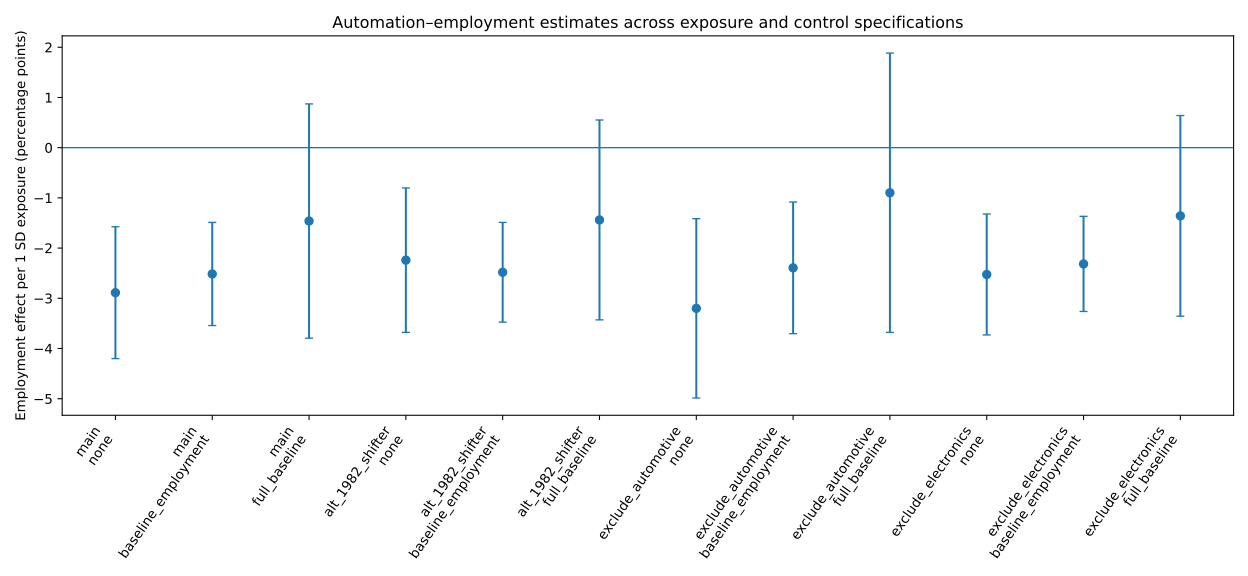
Static figure and accessible values follow.
Table 2. Main employment specification grid
| Treatment / shifter | Controls | Effect per 1 SD (pp) | First-stage F | p-value |
|---|---|---|---|---|
| Main | None | -2.89 | 62.6 | <0.001 |
| Main | Baseline employment | -2.52 | 96.5 | <0.001 |
| Main | Full baseline composition | -1.46 | 48.2 | 0.235 |
| 1982 external shifter | Baseline employment | -2.48 | 89.8 | <0.001 |
| Excluding automotive | Baseline employment | -2.39 | 38.1 | 0.002 |
| Excluding electronics | Baseline employment | -2.32 | 163.1 | <0.001 |
Note: Percentage-point effects scale each treatment by its observed province-level standard deviation. The attenuation under the full baseline vector is central to the qualified evidence label.
8.3 Few-cluster inference and leave-one-province-out stability
The province extension contains only 25 treatment clusters. Conventional asymptotics can therefore exaggerate certainty. Three additional exercises are used.
First, every leave-one-province-out estimate remains negative in the baseline-employment specification. The raw-exposure coefficient ranges from approximately -0.136 to -0.109. No single province creates the sign. The jackknife standard error is 0.0274, close to the conventional HC1 scale.
Second, a reduced-form permutation exercise randomizes the external shifter across the observed province outcomes. For the baseline-employment specification, the permutation p-value is 0.0084. With the full baseline composition vector, it rises to 0.259. The randomization exercise therefore tells the same story as the conventional standard errors: the simple negative relationship is unusually strong, but much of its statistical precision depends on how baseline composition is handled.
Third, an Anderson–Rubin-style inversion is used because it remains informative about weak-instrument uncertainty. The baseline-employment raw-exposure interval is approximately [-0.173, -0.071], or roughly [-3.53, -1.44] percentage points when scaled by the observed treatment standard deviation. The full-baseline interval expands across zero. First-stage weakness is therefore not the main problem; balance and coarse treatment-level variation are.
8.4 Attrition and demographic heterogeneity
Panel attrition is a plausible threat if workers facing adverse labor-market conditions become harder to recontact. A stabilized inverse-probability weight is estimated for continued observation and combined with the 2012 survey weight. Under that adjustment, the employment response remains negative at about -3.03 percentage points per standard deviation. Attrition therefore does not explain the main direction.
Exploratory subgroup estimates suggest larger displacement among older workers. The 45–60 baseline age group has an estimated response around -4.30 percentage points per standard deviation, compared with -1.45 points among workers aged 18–44. Estimates are negative for both men and women. The education split is less informative: workers with no more than nine years of schooling and those with at least twelve years have similarly negative point estimates. Because subgroup inference uses the same 25 province shocks and the interactions were not the primary estimand, these results are reported as exploratory rather than as a central claim.
8.5 Household total expenditure does not show a stable collapse
The household extension follows unique household transitions between 2012 and 2016. To avoid counting the same family change multiple times through different members, only one observation is retained for each matched household transition. Baseline household survey weights are used when aggregating outcomes to province level.
The strongest result is a null in the narrative sense: total household expenditure does not provide a stable negative response to automation exposure. The all-province total-PCE estimate is positive but imprecise. Excluding municipalities reverses its sign. Restricting the sample to provinces with at least 100 observed household transitions turns it positive again. Once baseline PCE is included, the coefficient is effectively zero. The confidence intervals do not justify a claim that robot exposure raised total consumption either. The correct statement is that the current design finds no stable directional effect on total PCE.
That finding is economically useful because it rejects a simplistic version of the Growth-to-Wallet story. A labor-market shock does not need to produce an immediate collapse in aggregate household spending. Families can adjust margins inside the consumption basket, delay housing-related commitments, use savings, borrow, change labor supply, or receive transfers.
8.6 Composition changes are more visible than the total
Food and housing shares show more stable movement. In the all-province specification, a one-standard-deviation increase in automation exposure is associated with a 2.75 percentage-point rise in food’s share of measured household consumption. The sign remains positive after municipalities are excluded and after the sample is restricted to provinces with at least 100 observed household transitions. The all-sample Benjamini–Hochberg q-value across the household outcome family is 0.016. Adding baseline food share reduces the magnitude but leaves the estimate positive and conventionally significant.
Housing expenditure share moves in the opposite direction. The all-province estimate implies a decline of about 0.97 percentage points per standard deviation. Its sign is stable across the main sample restrictions, and the baseline-housing-share specification remains negative. Precision weakens when municipalities are removed, where the conventional p-value is approximately 0.058.
Mortgage holding also declines in the all-province model, by roughly 3.15 percentage points per standard deviation. The estimate is large and survives multiple-testing correction in the full sample, but it becomes imprecise after municipalities are removed. Mortgage holding is therefore treated as a fragile balance-sheet result and is not used in the abstract.
Household expenditure-composition and mortgage responses
QUALIFIED / MORTGAGE FRAGILE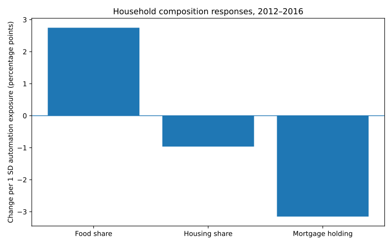
Static figure and accessible values follow.
Note: Food and housing shares are the two household composition outcomes emphasized in the main text. Mortgage holding is displayed for transparency but remains classified as fragile because precision collapses when municipalities are excluded.
Table 3. Household transition stability across geography/sample restrictions
| Outcome | All provinces | Excluding municipalities | Provinces with ≥100 household transitions | BH q, all provinces | Final label |
|---|---|---|---|---|---|
| Total PCE (log change coefficient) | +0.206 | -0.148 | +0.142 | 0.161 | Unsupported / unstable null |
| Food share | +2.75 pp/SD | positive, p=0.049 | positive, p=0.024 | 0.016 | Qualified |
| Housing share | -0.97 pp/SD | negative, p=0.058 | negative, p=0.001 | 0.016 | Qualified |
| Mortgage holding | -3.15 pp/SD | p=0.227 | p=0.006 | 0.014 | Fragile |
Note: Share/mortgage rows report the standardized treatment magnitude for the all-province model and direction/p-values for restricted samples. Total PCE is shown in its log-change coefficient scale because the sign itself is the relevant instability diagnostic.
These composition results are consistent with household defensiveness, but they do not identify a unique behavioral mechanism. Food share can rise because food expenditure is sticky while other categories fall, because relative prices change, or because household composition changes. Housing expenditure can respond to local property conditions that are correlated with industrial geography. The role of the empirical result is to show where the response appears in the data and where it does not: the composition margin is more stable than the total-spending margin.
8.7 Worker security as a within-person mechanism
The later CFPS waves provide a separate mechanism panel. Reported job security is standardized within each survey wave and related to worker outcomes using individual fixed effects and year fixed effects. This design removes time-invariant person heterogeneity but does not supply an external shock to subjective security; the estimates are therefore associations within workers over time.
In the 2016–2020 panel, a one-standard-deviation increase in reported security is associated with approximately 0.72 fewer weekly work hours, 1.14 percentage points greater labor-contract coverage, and 0.066 additional insurance categories. Those three associations survive Benjamini–Hochberg correction within the four-outcome worker family. Primary-job income is positive but imprecise.
Within-person job-security associations, 2016–2020
QUALIFIED ASSOCIATION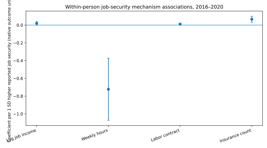
Static figure and accessible values follow.
The figure is intentionally labeled as a mechanism association rather than a technology-treatment effect. Subjective security has no external instrument in this module.
Table 4. Within-person job-security associations
| Outcome | 2016–2020 effect per 1 SD security | p-value | BH q | Pre-pandemic family result |
|---|---|---|---|---|
| Log primary-job income | +0.019 | 0.071 | 0.071 | Does not survive BH |
| Weekly hours | -0.723 hours | <0.001 | <0.001 | Does not survive BH family |
| Labor contract | +1.14 pp | 0.005 | 0.007 | Does not survive BH family |
| Insurance count | +0.066 | <0.001 | <0.001 | Does not survive BH family |
Interpretation: These are worker fixed-effects associations with standardized subjective security. They are not instrumented technology effects.
A stricter pre-pandemic window changes the strength of that evidence. Using only 2016 and 2018, the hours coefficient remains negative and contract and insurance coefficients remain positive, but none of the four outcomes survives family-wise BH correction at five percent. The mechanism evidence is therefore classified as pandemic-sensitive. It is consistent with the idea that employment quality contains margins hidden by employment status, but the paper does not claim that an exogenous increase in perceived security mechanically produces more contracts or insurance.
8.8 A household fixed-effects result that did not survive audit
An important final specification correction concerns household outcomes. A first-pass model attached each employed respondent’s job-security report to the income, consumption, and balance-sheet variables of that respondent’s household. If two eligible workers shared the same household, the identical household-year outcome could enter twice under different worker records. Person clustering did not eliminate that duplication.
The corrected design assigns at most one stable worker anchor to each household-year. The 2016–2020 corrected sample has 22,840 anchor person-waves, 9,351 anchor persons, and zero duplicate household-years. Under this design, the previously significant household-income and savings associations no longer clear conventional or multiple-testing thresholds. Household income per capita is positive but imprecise; savings is also positive but imprecise and weakens after current income is controlled. Total PCE, food share, housing share, education/entertainment share, and mortgage holding show no reliable relationship with subjective security.
This failed result is retained because it disciplines the paper’s mechanism claims. The CFPS data support a worker-side relationship between subjective security and several job attributes, but they do not provide strong within-person evidence that changes in reported security directly translate into household spending or balance-sheet changes. The household chapter must therefore rely on the separate automation-exposure transition evidence and on external theoretical and empirical literature for the broader smoothing mechanism.
8.9 What the original evidence establishes
The empirical evidence can now be stated without conditional placeholders.
- The published China robot benchmark is independently reproducible at the coefficient level.
- A new public-CFPS province extension yields a consistently negative automation-employment direction, but the causal magnitude is sensitive to baseline province composition and survey weighting.
- Total household PCE does not show a stable directional response in the same extension.
- Food and housing expenditure shares display more stable movement, suggesting that composition is a more informative margin than the headline total in this sample.
- Worker-level job-security associations reveal adjustment in hours, contracts, and insurance, although their statistical strength is concentrated in the 2020-inclusive panel.
- A direct household security-to-income/saving result fails after household-year duplication is removed.
The Growth-to-Wallet framework therefore survives as a useful organizing device, but its strongest empirical version is narrower: technology exposure is associated with labor-market displacement, while household adjustment appears more clearly in expenditure composition than in total spending. The data do not support a claim that this single channel explains China’s weak household demand in 2026.
Table 5. Final evidence classification
| Result | Classification | Headline use |
|---|---|---|
| Published Giuntella–Lu–Wang coefficient replication | ROBUST / REPRODUCED | Yes |
| Original 2012–2016 automation exposure → employment | QUALIFIED | Yes, with identification caveat |
| Larger response among older workers | EXPLORATORY | Appendix / secondary |
| Total household PCE | UNSUPPORTED / UNSTABLE NULL | Yes, as a non-result |
| Food share response | QUALIFIED | Yes |
| Housing share response | QUALIFIED | Yes |
| Mortgage holding | FRAGILE | Secondary |
| Job security → worker hours/contracts/insurance | QUALIFIED / PANDEMIC-SENSITIVE | Mechanism evidence |
| Job security → household income/savings | UNSUPPORTED AFTER DEDUPLICATION | Yes, as audit failure |
| Job security → household consumption | UNSUPPORTED | Secondary |
9. Robustness, Falsification, and Interpretation Boundaries
9.1 Classification rule
Every empirical result is assigned one of four statuses before it enters the abstract or conclusion: robust/reproduced, qualified, fragile/exploratory, or unsupported. The classification is based on sign stability, magnitude stability, inference appropriate to the treatment level, baseline balance, alternative exposure definitions, sample restrictions, multiple-testing adjustment, and whether the identifying variation can reasonably support causal language.
The benchmark Table 2 coefficient replication is robust/reproduced. The original province automation-employment result is qualified. Food-share and housing-share responses are qualified household results. Mortgage holding is fragile. The direct total-PCE response and the deduplicated household-security outcomes are unsupported as directional claims.
9.2 Alternative robot shifters and dominant sectors
The first robustness question is whether the employment result depends on one construction of the external instrument. Replacing the main 2000-share European shifter with the alternative 1982-share shifter preserves the negative sign. In the baseline-employment province specification, the effect is -2.48 percentage points per standard deviation rather than -2.52 under the main shifter.
The second question is whether a robot-intensive sector mechanically dominates the treatment. The public exposure file permits variants excluding automotive and excluding electronics. Both produce negative baseline-controlled effects: approximately -2.39 and -2.32 percentage points per standard deviation, respectively. Their first stages remain usable. This matters because the published Rotemberg-weight diagnostics show substantial weight on electronics and other selected sectors. The extension is therefore not a one-sector arithmetic artifact.
These checks do not solve the central identification problem. They show that the negative direction is not unique to the main shifter or to the two most obvious robot-intensive sectors.
9.3 Baseline composition is the main weakness
The main external shifter is strongly related to several baseline characteristics across the 25 observed provinces. The correlation is approximately 0.48 with mean age, 0.64 with education years, and 0.58 with urban share. HC1 tests remain small after within-shifter Benjamini–Hochberg adjustment. These are not trivial correlations in a 25-unit treatment sample.
Baseline balance of the main external shifter
IDENTIFICATION DIAGNOSTIC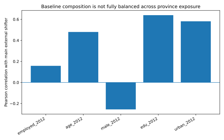
Static figure and accessible values follow.
The diagnostic is shown because it governs the paper’s causal language: baseline education, urbanization, and age are materially related to the main shifter in the observed CFPS province sample.
The consequence appears directly in the coefficient path. The no-control and baseline-employment province specifications imply effects near -2.9 and -2.5 percentage points per standard deviation. Adding age, sex composition, education, and urbanization reduces the estimate to roughly -1.5 points and makes it statistically imprecise. The sign remains negative under every leave-one-province-out version of the full specification, but the confidence interval allows both a modest negative effect and a small positive value.
The paper therefore refuses a common but misleading robustness move: controls are not dismissed simply because they reduce significance. The balance test was specified to detect exactly this problem. Once it appears, the narrower result governs the causal language.
The result also survives several sample-support restrictions in the baseline-employment specification. Excluding Beijing, Tianjin, Shanghai, and Chongqing leaves 21 provinces and an estimated -1.72 percentage points per standard deviation (p=0.038; first-stage F=87.0). Requiring at least 100 linked persons per province gives -2.58 points; thresholds of 200 and 300 give about -2.22 points. Even the 12 provinces with at least 500 linked persons produce -3.54 points. The full baseline composition specification, however, remains imprecise in each of these restricted samples and is close to zero in the highest-support subset. This pattern strengthens confidence in the negative direction under parsimonious adjustment while reinforcing that the fully adjusted causal magnitude is unresolved.
Table 6. Sample-support sensitivity of the main employment specification
| Province sample | N provinces | Baseline-employment effect (pp/SD) | p-value | Full-baseline effect (pp/SD) | p-value |
|---|---|---|---|---|---|
| All observed | 25 | -2.52 | <0.001 | -1.46 | 0.235 |
| Excluding municipalities | 21 | -1.72 | 0.038 | -0.26 | 0.821 |
| At least 100 linked persons | 24 | -2.58 | <0.001 | -0.97 | 0.452 |
| At least 200 linked persons | 22 | -2.22 | <0.001 | -0.64 | 0.634 |
| At least 300 linked persons | 20 | -2.22 | <0.001 | +0.81 | 0.546 |
| At least 500 linked persons | 12 | -3.54 | 0.001 | -0.03 | 0.986 |
A province-size-weighted specification points the same way: -3.32 points with baseline employment and -0.19 points with the full baseline vector. These weighting exercises are sensitivity checks, not a search for a preferred significant estimand.
9.4 Survey weights and individual-level estimation
The province aggregate gives each observed province equal weight. A second estimand uses individual long differences and clusters the covariance at the province treatment level. A third applies the 2012 CFPS individual survey weight.
The unweighted person-level estimates remain negative and conventionally significant through the full baseline control set. Survey weighting produces smaller main-shifter estimates and wider intervals. With baseline employment, the weighted main-shifter estimate is about -2.22 percentage points per standard deviation; with the full baseline vector it is about -1.59 points. Neither clears a five-percent conventional threshold. The alternative 1982 shifter remains larger and statistically distinguishable from zero under the same weighting.
This variation is substantive. Equal-province, respondent-weighted, and alternative-shifter specifications target different weighted combinations of local treatment effects. The paper reports them together rather than treating the national-sounding weighted result as automatically superior or the strongest unweighted result as automatically preferred.
9.5 Few treatment clusters
Twenty-five treatment clusters are too few for casual reliance on individual-level heteroskedasticity-robust standard errors. All person-level IV estimates cluster at province. The province aggregate additionally uses leave-one-province-out, jackknife, permutation, and Anderson–Rubin-style diagnostics.
For the baseline-employment model, the leave-one-province-out sign is negative in every iteration and the reduced-form permutation p-value is 0.0084. The Anderson–Rubin interval excludes zero. Under the full baseline composition vector, both the permutation test and the Anderson–Rubin interval cease to reject zero. The inference stress therefore confirms rather than resolves the balance sensitivity.
9.6 Attrition
Longitudinal household surveys can lose respondents selectively. The probability of remaining observed through 2016 is modeled from baseline information, producing stabilized attrition weights that are combined with the 2012 survey weight. The attrition-adjusted province estimate remains negative at roughly -3.03 percentage points per standard deviation.
This result makes selective disappearance an unlikely explanation for the sign. It does not prove that attrition is ignorable: inverse-probability weighting depends on observed predictors. Unobserved migration or labor shocks can still affect survey retention.
9.7 Household outcome multiplicity
The household transition module tests several outcomes: income, total PCE, food expenditure, education/entertainment expenditure, savings, expenditure shares, housing share, and mortgage holding. Because a large outcome menu can generate accidental significance, Benjamini–Hochberg q-values are reported across the all-province household family.
Food share, housing share, mortgage holding, and log food expenditure clear a five-percent BH threshold in the all-province family. The geography restrictions separate them further. Food share remains positive with p<0.05 when municipalities are removed and when low-count provinces are removed. Housing share retains the same sign and remains strong in the minimum-household-count sample, with a marginal p-value after municipalities are excluded. Mortgage holding loses precision sharply without municipalities. Log food expenditure also weakens without municipalities.
The paper therefore emphasizes food share and housing share rather than whichever individual household coefficient has the smallest p-value.
9.8 Total consumption as an unstable null
A non-significant coefficient does not automatically prove zero effect. The total-PCE result is better described as an unstable null. Its point estimate changes sign across defensible samples, and the baseline-outcome control brings it close to zero with a wide interval. The design therefore cannot rule out economically meaningful positive or negative responses.
The paper’s claim is limited to the absence of a stable directional total-PCE result. It does not state that households perfectly smooth every automation shock.
9.9 Pandemic sensitivity in job-quality mechanisms
The 2020 CFPS wave occurred under exceptional labor-market and public-health conditions. The job-security mechanism is therefore estimated both for 2016–2018 and for 2016–2020.
The 2020-inclusive panel produces clear within-person relationships for weekly hours, labor-contract coverage, and insurance count after multiple-testing adjustment. In the 2016–2018 panel, those directions remain economically coherent but the four-outcome family does not survive BH correction at five percent. Any interpretation of the job-security module must therefore acknowledge that part of its statistical strength comes from variation present by 2020.
This result is not discarded; it changes the label. The job-security module is mechanism evidence that is informative about margins of adjustment, with pandemic-period sensitivity, rather than a timeless structural coefficient.
9.10 Household-year duplication audit
The most consequential specification audit is a negative one. Linking worker security to household outcomes at the respondent level duplicates a household-year whenever multiple eligible workers live together. That design can understate uncertainty and can make household-level associations appear stronger than they are.
The corrected unique-anchor sample contains no duplicate household-years. After the correction, household income, savings, total PCE, expenditure shares, and mortgage holding do not survive multiple-testing adjustment. The prior positive household income/savings results are removed from the paper.
This is treated as a successful falsification exercise. A result that depends on an invalid repeated-outcome construction does not become part of the evidence simply because its sign matches the theory.
9.11 Geography and external validity
Public CFPS geography is coarser than the published city-level robot design. The province aggregation averages heterogeneous local shocks and yields only 25 observed treatment units in the linked sample. It also changes the estimand from a city-level worker exposure effect to an exposure-weighted province relationship among the observed CFPS population.
The paper consequently does not describe the new extension as a nationally representative causal estimate of robots on Chinese employment. Its role is replication-consistent external evidence and a bridge to household outcomes that are unavailable in the public aggregate city data.
9.12 What would upgrade the evidence
Three additions would materially strengthen the causal chapter.
- Authorized sub-provincial CFPS geography would allow the household extension to inherit the published city-level treatment architecture directly.
- A licensed later IFR panel would allow genuine time-varying automation exposure after 2016 rather than freezing or extrapolating the historical shock.
- Shock-level inference with the full underlying industry-shock structure would be preferable to treating 25 provinces as the only effective source of uncertainty.
Until those conditions are met, the paper keeps the benchmark replication and the province household extension distinct.
10. Mechanisms: Job Quality, Household Smoothing, and the Limits of the Current Data
10.1 Adjustment below the employment indicator
The automation result motivates a second question: what happens among workers who remain employed? CFPS job-security, hours, contract, and insurance variables make it possible to observe margins that a binary employment indicator misses.
Within-person estimates over 2016–2020 associate a one-standard-deviation increase in reported job security with fewer weekly hours, greater contract coverage, and more work-related insurance categories. The signs are coherent with a job-quality interpretation in which security is partly reflected in formal protections and work intensity. Yet reported security is subjective. A wage increase, promotion, employer change, family shock, or local labor-market improvement can alter both security perceptions and observed job conditions. Person fixed effects remove stable individual traits but do not remove those time-varying common causes.
The pre-pandemic sensitivity further limits interpretation. Using only 2016 and 2018, the same broad directions appear, but the outcome family no longer survives multiple-testing correction. The job-quality evidence therefore supports the proposition that workers adjust on intensive and contractual margins; it does not identify a causal security shock.
10.2 Why total consumption can remain smooth
The household transition estimates show no stable directional response of total PCE to automation exposure. This is compatible with standard consumption-smoothing models. A household facing weaker employment prospects can preserve current expenditure by drawing down liquid balances, borrowing, reallocating labor supply, receiving transfers, or postponing large commitments. The absence of a total-PCE coefficient is therefore not evidence that labor risk is irrelevant.
The more stable movement in food and housing shares points toward internal reallocation. Food is relatively difficult to postpone. Housing-related spending and mortgage decisions contain larger adjustment margins. A rise in food share can occur even if nominal food expenditure changes little, provided more deferrable categories slow. A fall in housing share can reflect delayed housing expenditure, different rental or mortgage decisions, or local property-market conditions.
The current data cannot cleanly separate those channels. The composition result is therefore treated as a behavioral signature rather than as a structural marginal propensity to consume.
10.3 Balance sheets: suggestive, not settled
Mortgage holding falls in the all-province automation specification, but the result is sensitive to municipality exclusion. Savings does not produce a stable automation estimate. The corrected job-security fixed-effects design also fails to show robust savings or mortgage responses.
The paper therefore avoids a strong claim that Chinese households respond to automation primarily by deleveraging or accumulating deposits. The macro fact of rising household deposits in 2026 is used as external context, not as a mechanical extrapolation from the 2012–2016 CFPS shock.
10.4 The failed direct household-security channel
The unique-anchor correction changes the interpretation of the household mechanism. Once each household-year contributes only once, changes in subjective worker security no longer have a statistically reliable direct association with household income, total consumption, savings, or expenditure shares.
This failure narrows the Growth-to-Wallet mechanism. The data provide stronger evidence for the technology-to-employment link and for household composition changes under geographic exposure than for a continuous security-belief-to-consumption coefficient inside the later panel.
That distinction is useful. It prevents the framework from becoming a chain in which every arrow is assumed to exist because the overall narrative is attractive. Some links are supported, some are qualified, and some remain unmeasured.
10.5 What remains of the Growth-to-Wallet framework
The empirical framework can now be written with evidence labels:
\[ Automation\ Exposure \xrightarrow{\text{qualified negative employment evidence}} Labor\ Market \xrightarrow{\text{worker mechanism associations}} Job\ Quality/Security \xrightarrow{\text{not directly identified}} Household\ Expectations \xrightarrow{\text{qualified composition evidence}} Spending\ Mix. \]
The discontinuities are part of the result. The current evidence does not support multiplying estimated coefficients into a single structural pass-through number. It supports a map of where transmission appears strong, where it becomes uncertain, and where household smoothing breaks the simple relationship between labor shocks and headline consumption.
10.6 Implications for the 2026 macro puzzle
The historical automation evidence cannot be used to claim that robots caused China’s weak household demand in 2026. The time periods differ, the industrial-policy environment differs, the property market has changed, and the current economy contains many shocks absent from the 2012–2016 sample.
What the evidence can do is discipline the interpretation of a K-shaped economy. Strong production or technology indicators do not guarantee equally strong employment absorption. Worker adjustment can occur through hours and formal job attributes. Household expenditure can remain smooth at the total while its composition changes. These mechanisms make it empirically plausible for a production-heavy recovery to coexist with household caution without requiring a one-to-one causal story from any single technology shock.
11. Policy Interpretation
The empirical results narrow the policy interpretation. They do not support a claim that China’s household-demand problem can be solved by reversing automation, nor do they show that historical robot exposure caused the 2026 consumption slowdown. They support a more specific point: productive upgrading can generate worker displacement without an immediate fall in total household expenditure, while expenditure composition and job-quality margins adjust underneath the headline totals.
11.1 Labor absorption belongs next to productivity
The published robot benchmark and the new CFPS province extension both point toward a negative employment margin under higher historical automation exposure. The original extension is qualified, yet its sign survives alternative shifters, sector exclusions, attrition adjustment, and leave-one-province-out estimation. That makes worker transition a policy-relevant margin even when the exact causal magnitude remains uncertain.
Technology policy therefore benefits from measuring labor absorption directly. Output, productivity, capacity, export share, and robot density describe what production can do. They do not reveal how many workers move into better jobs, how long displacement lasts, or whether replacement work carries comparable pay, security, and insurance.
Training is useful only when it connects to realistic labor demand. A retraining program that awards certificates without producing credible employer demand does little for worker outside options. More informative metrics include post-training employment, earnings, occupation switching, geographic mobility, and retention after six or twelve months.
11.2 Household policy should watch composition as well as totals
The CFPS household transition results do not show a stable decline in total PCE. Food share rises and housing share falls more consistently. That result argues against using one aggregate consumption number as the sole household-stress indicator.
A household can preserve its total spending while becoming more defensive. It can delay housing-related expenditure, avoid a mortgage commitment, reduce deferrable categories, or use financial buffers. Policy evaluation should therefore track expenditure composition, new borrowing, liquid assets, debt service, and large durable commitments alongside retail totals.
The mortgage result in this paper is fragile and should not be used as a policy coefficient. Its instability is itself useful: property-market geography can dominate household balance-sheet estimates, so labor and property mechanisms need to be separated rather than blended into one explanation.
11.3 Social insurance affects the cost of transition
The paper does not identify a direct causal effect of subjective job security on household consumption. The corrected unique-anchor estimates remove the earlier apparent household income and savings significance. That failed result prevents an easy claim that improving subjective security by one standard deviation would mechanically raise spending by a known amount.
Social insurance still matters economically because it changes the cost of labor-market transitions. Unemployment insurance, health coverage, pension portability, and credible income support reduce the private resources a household must reserve against a bad employment state. The relevant evaluation question is therefore not only whether transfers raise current expenditure, but whether they reduce the need for costly self-insurance and permit workers to search for better matches rather than accepting the first available low-quality job.
11.4 Job quality is visible in hours, contracts, and insurance
The within-person CFPS mechanism panel shows that changes in reported job security move with weekly hours, formal contracts, and insurance coverage in the 2020-inclusive sample. The pre-pandemic evidence is weaker, so these coefficients are not structural policy effects. They nonetheless demonstrate why binary employment is a poor complete measure of adjustment.
A worker can remain employed while working longer hours, losing formal coverage, or accepting a less secure arrangement. Conversely, formalization can improve even when income growth is modest. Labor-market monitoring should therefore place contract status, social insurance, working time, and job-to-job transitions beside unemployment.
11.5 Worker outside options remain central
The broader literature reviewed in this paper shows why outside options affect who captures productivity gains. Mobility costs, limited vacancies, occupational specificity, geographic restrictions, and employer concentration can weaken the bargaining position of workers even when firms become more productive.
Policies that expand credible outside options can operate through several concrete channels: portable benefits, reliable vacancy information, lower barriers to occupational transfer, lower geographic mobility costs, targeted enforcement of non-compete restrictions, and accessible dispute resolution. The objective is not to maximize turnover. It is to reduce the cost of saying no to a bad match.
11.6 Production rebalancing and household rebalancing remain distinct
China can improve the technological composition of production faster than it improves household demand. The historical micro evidence makes that divergence plausible without proving a single contemporary cause. A production system can become more automated and competitive while some workers face displacement and households reallocate expenditure defensively.
The appropriate policy target is therefore stronger transmission from productive gains into stable household resources. That target can coexist with continued technological upgrading. The empirical question is whether productivity gains generate replacement work, earnings, security, and insurance quickly enough to keep household balance sheets from carrying the transition alone.
12. Conclusion
This paper began with a distributional question: who captures growth when production becomes more capital- and technology-intensive? The answer cannot be read from output growth alone. It requires tracing the route from technology into employment, job quality, income, household risk, and spending.
The empirical work produces four main findings.
First, the published China robot benchmark passes an independent analytical replication gate. All six headline Table 2 2SLS coefficients reproduce at the displayed three-decimal precision from the public final analysis files. This establishes a reliable external benchmark: historical local robot exposure in China generated meaningful worker adjustment, including lower employment and hourly earnings and higher hours among workers who remained employed.
Second, the new public-CFPS province extension points in the same employment direction but with an important qualification. One standard deviation of additional 2010–2014 robot exposure corresponds to an employment decline of roughly 2.5 percentage points in the baseline-employment province model. The sign remains negative under the 1982 external shifter, after removing automotive or electronics exposure, after attrition adjustment, and in every leave-one-province-out estimate. Yet the main shifter is correlated with baseline age, education, and urbanization. Once the full baseline composition vector is included, the equal-weight province point estimate falls to roughly -1.5 percentage points and the confidence interval crosses zero. Survey weighting also weakens the main-shifter precision. The result therefore enters the paper as qualified evidence rather than an unconditional causal estimate.
Third, household adjustment appears more clearly in composition than in total spending. Total PCE does not show a stable directional response to automation exposure. Food share rises by about 2.75 percentage points per standard deviation in the all-province estimate, while housing share falls by about 0.97 points; both directions survive the main sample restrictions, although the housing result becomes marginal without municipalities. Mortgage holding falls in the full sample but is too geography-sensitive for a headline claim. These results are consistent with defensive reallocation and smoothing, while leaving property conditions and other local shocks as serious competing explanations.
Fourth, the later job-security panel teaches a useful lesson about mechanism evidence. Within workers, reported security moves with hours, contract coverage, and insurance in the 2016–2020 panel, but the pre-pandemic evidence is weaker. More importantly, a direct household security-to-income/savings result disappears after the analysis prevents duplicate family-year outcomes. The paper therefore rejects its own earlier household mechanism estimate rather than preserving a coefficient that depended on a flawed unit of observation.
Together, these results sharpen the Growth-to-Wallet framework. The empirical chain is not a sequence of coefficients that can be multiplied into one national pass-through number. It is a map with strong links, weak links, and missing links. Historical automation exposure has credible worker consequences. The public-CFPS extension provides qualified evidence of employment displacement. Household totals are smoother than the labor outcome, while selected expenditure shares move more visibly. Subjective worker security contains information about job conditions, but it does not supply a clean causal bridge to household spending in the current data.
That pattern matters for the interpretation of China’s 2026 economy. Strong high-technology production and exports can coexist with household caution because the route from production to household purchasing power is mediated by employment absorption, bargaining conditions, transition risk, property balance sheets, and insurance. The historical evidence makes that coexistence plausible. It does not establish that robot adoption caused the current macroeconomic divergence.
The paper therefore stops short of a monocausal explanation. Property adjustment, demographics, fiscal composition, external demand, corporate profitability, and credit conditions remain competing mechanisms. The current macro figures identify the puzzle; the historical micro evidence identifies several channels through which that puzzle can arise.
The research also produces a clear next frontier. Authorized sub-provincial CFPS geography would permit household outcomes to inherit the stronger published local robot design. Later licensed IFR data would allow technology exposure to extend genuinely beyond 2016. Until those inputs exist, the evidence should remain calibrated to what the public data can identify.
The final conclusion is concrete. Productive upgrading can succeed statistically before it succeeds in the household budget. Whether growth reaches the wallet depends on what happens between the factory, the job, and the family balance sheet. Measuring those intermediate steps is necessary if industrial upgrading and household rebalancing are expected to move together.
Data and Reproducibility Note
The empirical build uses public CFPS waves for 2012, 2014, 2016, 2018, and 2020, public analytical materials from the Giuntella–Lu–Wang robot replication package, and a province aggregation of the public robot-exposure series. CFPS raw microdata and row-level derived data are not redistributed.
The public replication package accompanying this paper contains:
- CFPS harmonization and audit code;
- a public variable crosswalk;
- aggregate province long-difference data;
- robot-exposure variant data at province level where redistribution is permitted;
- regression and inference tables;
- result-classification metadata;
- publication figures and machine-readable aggregate result files.
It excludes CFPS .dta files, private serialized panels, row-level person records, and household microdata. Reproducing the CFPS results requires users to obtain CFPS data through the official data-access process and place them in the local paths described by the configuration documentation.
The independent Giuntella–Lu–Wang exercise reproduces the six headline Table 2 coefficient values from the supplied public final analysis file. Native execution of the authors’ Stata covariance workflow remains a separate software-reproduction task and is not represented as complete.
The publication date is 19 August 2026. Contemporary macroeconomic statistics are dated explicitly in the paper and should be refreshed if the article is republished after newer official or international releases become available.
SOURCES & DATA
References
Acemoglu, D. and Restrepo, P. (2019). ‘Automation and New Tasks: How Technology Displaces and Reinstates Labor’, Journal of Economic Perspectives, 33(2), pp. 3–30. Earlier working-paper version: NBER Working Paper 25684. https://www.nber.org/papers/w25684
Acemoglu, D. and Restrepo, P. (2020). ‘Robots and Jobs: Evidence from US Labor Markets’, Journal of Political Economy, 128(6), pp. 2188–2244. Earlier working-paper version: NBER Working Paper 23285. https://www.nber.org/papers/w23285
Azar, J., Marinescu, I. and Steinbaum, M. (2022). ‘Labor Market Concentration’, Journal of Human Resources, 57(S), pp. S167–S199. Related working paper: NBER Working Paper 24147. https://www.nber.org/papers/w24147
Benmelech, E., Bergman, N. K. and Kim, H. (2022). ‘Strong Employers and Weak Employees: How Does Employer Concentration Affect Wages?’, Journal of Human Resources, 57(S), pp. S200–S250. Earlier working paper: NBER Working Paper 24307. https://www.nber.org/papers/w24307
Blanchard, O. J. and Giavazzi, F. (2005). Rebalancing Growth in China: A Three-Handed Approach. MIT Department of Economics Working Paper 05-32. https://dspace.mit.edu/entities/publication/b7a9b28f-46aa-47da-8968-9c36db932b24
Borusyak, K., Hull, P. and Jaravel, X. (2022). ‘Quasi-Experimental Shift-Share Research Designs’, Review of Economic Studies, 89(1), pp. 181–213. https://academic.oup.com/restud/article/89/1/181/6294942
Borusyak, K., Jaravel, X. and Spiess, J. (2024). ‘Revisiting Event-Study Designs: Robust and Efficient Estimation’, Review of Economic Studies, 91(6), pp. 3253–3285. https://academic.oup.com/restud/article/91/6/3253/7601390
Browning, M. and Crossley, T. F. (2001). ‘The Life-Cycle Model of Consumption and Saving’, Journal of Economic Perspectives, 15(3), pp. 3–22. https://www.aeaweb.org/articles?id=10.1257/jep.15.3.3
Carroll, C. D. (1997). ‘Buffer-Stock Saving and the Life Cycle/Permanent Income Hypothesis’, Quarterly Journal of Economics, 112(1), pp. 1–55.
Chamon, M. D. and Prasad, E. S. (2010). ‘Why Are Saving Rates of Urban Households in China Rising?’, American Economic Journal: Macroeconomics, 2(1), pp. 93–130. https://www.aeaweb.org/articles?id=10.1257/mac.2.1.93
Chamon, M., Liu, K. and Prasad, E. (2013). ‘Income Uncertainty and Household Savings in China’, Journal of Development Economics, 105, pp. 164–177. https://doi.org/10.1016/j.jdeveco.2013.07.014
Cooper, R. and Zhu, G. (2017). Household Finance in China. NBER Working Paper 23741. https://www.nber.org/papers/w23741
Dahl, G. B. and Knepper, M. (2026). ‘Why Is Workplace Sexual Harassment Underreported? The Value of Outside Options amid the Threat of Retaliation’, American Economic Review, 116(3), pp. 897–933. https://www.aeaweb.org/articles?id=10.1257/aer.20221703
Fang, H., Li, M. and Lu, G. (2025; revised July 2026). Decoding China’s Industrial Policies. NBER Working Paper 33814. https://www.nber.org/papers/w33814
Gallagher, M., Giles, J., Park, A. and Wang, M. (2013). China’s 2008 Labor Contract Law: Implementation and Implications for China’s Workers. IZA Discussion Paper 7555. https://www.iza.org/publications/dp/7555/
Giuntella, O., Lu, Y. and Wang, T. (2022). How Do Workers and Households Adjust to Robots? Evidence from China. NBER Working Paper 30707. https://www.nber.org/papers/w30707
Giuntella, O., Lu, Y. and Wang, T. (2025). ‘How Do Workers Adjust to Robots? Evidence from China’, Economic Journal, 135(666), pp. 637–652. https://academic.oup.com/ej/article/135/666/637/7789857
Giuntella, O., Lu, Y. and Wang, T. (2024). Replication Package for: How do Workers Adjust to Robots? Evidence from China. Zenodo, version v1. https://doi.org/10.5281/zenodo.13760908
Goldsmith-Pinkham, P., Sorkin, I. and Swift, H. (2020). ‘Bartik Instruments: What, When, Why, and How’, American Economic Review, 110(8), pp. 2586–2624. https://www.aeaweb.org/articles?id=10.1257/aer.20181047
He, H., Huang, F., Liu, Z. and Zhu, D. (2018). ‘Breaking the “Iron Rice Bowl”: Evidence of Precautionary Savings from the Chinese State-Owned Enterprises Reform’, Journal of Monetary Economics, 94, pp. 94–113.
Institute of Social Science Survey, Peking University (2012). China Family Panel Studies 2012 Public-Use Data and Documentation. https://www.isss.pku.edu.cn/cfps/
Institute of Social Science Survey, Peking University (2014). China Family Panel Studies 2014 Public-Use Data and Documentation. https://www.isss.pku.edu.cn/cfps/
Institute of Social Science Survey, Peking University (2016). China Family Panel Studies 2016 Questionnaires and Public-Use Data. https://www.isss.pku.edu.cn/cfps/
Institute of Social Science Survey, Peking University (2018). China Family Panel Studies 2018 Questionnaires. https://www.isss.pku.edu.cn/cfps/
Institute of Social Science Survey, Peking University (2020). China Family Panel Studies 2020 Questionnaires. https://www.isss.pku.edu.cn/cfps/
Institute of Social Science Survey, Peking University (2026). CFPS Data User Agreement, Data-Sharing Regulations, and Restricted Data Guidelines. https://www.isss.pku.edu.cn/cfps/en/data/DataUserAgreement/index.htm
International Federation of Robotics (2026). World Robotics — Industrial Robots / Database Documentation. https://ifr.org/worldrobotics/
International Monetary Fund (2026). People’s Republic of China: 2025 Article IV Consultation—Press Release; Staff Report; and Statement by the Executive Director for the People’s Republic of China. IMF Country Report No. 26/044, 18 February 2026. https://doi.org/10.5089/9798229038911.002
Kessler, J. B., Low, C. and Sullivan, C. D. (2019). ‘Incentivized Resume Rating: Eliciting Employer Preferences without Deception’, American Economic Review, 109(11), pp. 3713–3744. https://www.aeaweb.org/articles?id=10.1257/aer.20181714
Liu, J., Cai, H. and Lin, C. (2025). ‘Competition in the Labor Market: The Wage Effect of Employer Concentration in China’, Industrial Relations: A Journal of Economy and Society, 64(3), pp. 343–379. Earlier version: IZA Discussion Paper 17226. https://www.iza.org/publications/dp/17226/
Liu, J., Cai, H. and Lin, C. (2026). ‘Correction to “Competition in the Labor Market: The Wage Effect of Employer Concentration in China”’, Industrial Relations: A Journal of Economy and Society, 65(1), p. 100. https://doi.org/10.1111/irel.70001
Ministry of Justice of the People’s Republic of China / Legal Daily (2024). ‘Employment Background Checks Should Not Become Privacy Fishing’. https://legalinfo.moj.gov.cn/pub/sfbzhfx/zhfxfzzx/fzzxyw/202403/t20240314_496129.html
National Bureau of Statistics of China (2026a). ‘National Economy Maintained Steady Momentum with Innovation-driven and High-quality Development in the First Seven Months’, 17 August 2026. https://www.stats.gov.cn/english/PressRelease/202608/t20260817_1965057.html
People’s Bank of China (2026). ‘Financial Statistics Report (July 2026)’, 14 August 2026. https://www.pbc.gov.cn/en/3688247/3688978/3709137/2026081815052522832/index.html
Rambachan, A. and Roth, J. (2023). ‘A More Credible Approach to Parallel Trends’, Review of Economic Studies, 90(5), pp. 2555–2591. https://academic.oup.com/restud/article/90/5/2555/7039335
Song, Z., Storesletten, K. and Zilibotti, F. (2011). ‘Growing Like China’, American Economic Review, 101(1), pp. 196–233. https://www.aeaweb.org/articles?id=10.1257/aer.101.1.196
Supreme People’s Court of the People’s Republic of China (2024). ‘First Batch of Guiding Cases on Labor Disputes in New Forms of Employment’, 23 December 2024. https://www.court.gov.cn/zixun/xiangqing/450651.html
Supreme People’s Court of the People’s Republic of China (2025). ‘Interpretation (II) on Several Issues Concerning the Application of Law in the Trial of Labor Dispute Cases’, released 1 August 2025, effective 1 September 2025. https://www.court.gov.cn/zixun/xiangqing/472691.html
Supreme People’s Court of the People’s Republic of China (2026a). Press conference discussion of digital / “invisible overtime”, 2 March 2026. https://www.court.gov.cn/zixun/xiangqing/490761.html
Supreme People’s Court of the People’s Republic of China (2026b). Work Report of the Supreme People’s Court, March 2026. https://www.court.gov.cn/zixun/xiangqing/492921.html
Survey and Research Center for China Household Finance, Southwestern University of Finance and Economics (2026). CHFS Data Application and Data Use Documentation. https://chfs.swufe.edu.cn/sjzx/sjsq.htm
World Bank (2026). China Economic Update: Rebalancing Growth. July 2026. https://www.worldbank.org/en/news/press-release/2026/07/07/rebalancing-growth-china-economic-update
Zhang, L. (2016). Rebalancing in China—Progress and Prospects. IMF Working Paper 16/183. https://www.imf.org/external/pubs/ft/wp/2016/wp16183.pdf
Direct Source Links
The list below is provided for web publication and machine-readable integration. It supplements the author–date bibliography above with direct source URLs.
National Economy Maintained Steady Momentum with Innovation-driven and High-quality Development in the First Seven Months — National Bureau of Statistics of China — https://www.stats.gov.cn/english/PressRelease/202608/t20260817_1965057.html
Financial Statistics Report (July 2026) — People’s Bank of China — https://www.pbc.gov.cn/en/3688247/3688978/3709137/2026081815052522832/index.html
China Economic Update: Rebalancing Growth — World Bank — https://www.worldbank.org/en/news/press-release/2026/07/07/rebalancing-growth-china-economic-update
People’s Republic of China: 2025 Article IV Consultation—Press Release; Staff Report; and Statement by the Executive Director for the People’s Republic of China — International Monetary Fund — https://www.imf.org/en/publications/cr/issues/2026/02/17/peoples-republic-of-china-2025-article-iv-consultation-press-release-staff-report-and-574028 — DOI: https://doi.org/10.5089/9798229038911.002
Press conference discussion of digitally mediated / invisible overtime — Supreme People’s Court of the People’s Republic of China — https://www.court.gov.cn/zixun/xiangqing/490761.html
Interpretation (II) on Several Issues Concerning the Application of Law in the Trial of Labor Dispute Cases — Supreme People’s Court of the People’s Republic of China — https://www.court.gov.cn/zixun/xiangqing/472691.html
First guiding cases on labor disputes in new forms of employment — Supreme People’s Court of the People’s Republic of China — https://www.court.gov.cn/zixun/xiangqing/450651.html
How do Workers Adjust to Robots? Evidence from China — Osea Giuntella, Yi Lu, Tianyi Wang — https://academic.oup.com/ej/article-abstract/135/666/637/7789857 — DOI: https://doi.org/10.1093/ej/ueae086
Replication Package for: How do Workers Adjust to Robots? Evidence from China — Osea Giuntella, Yi Lu, Tianyi Wang — https://zenodo.org/records/13760908 — DOI: https://doi.org/10.5281/zenodo.13760908
How Do Workers and Households Adjust to Robots? Evidence from China — Osea Giuntella, Yi Lu, Tianyi Wang — https://www.nber.org/papers/w30707
Automation and New Tasks: How Technology Displaces and Reinstates Labor — Daron Acemoglu, Pascual Restrepo — https://www.nber.org/papers/w25684
Robots and Jobs: Evidence from US Labor Markets — Daron Acemoglu, Pascual Restrepo — https://www.nber.org/papers/w23285 — DOI: https://doi.org/10.1086/705716
Competition in the Labor Market: The Wage Effect of Employer Concentration in China — J. Liu, H. Cai, C. Lin — https://onlinelibrary.wiley.com/doi/10.1111/irel.12377 — DOI: https://doi.org/10.1111/irel.12377
Correction to Competition in the Labor Market: The Wage Effect of Employer Concentration in China — https://onlinelibrary.wiley.com/doi/10.1111/irel.70001 — DOI: https://doi.org/10.1111/irel.70001
Decoding China’s Industrial Policies — Hanming Fang, Ming Li, Guangli Lu — https://www.nber.org/papers/w33814
Growing Like China — Zheng Song, Kjetil Storesletten, Fabrizio Zilibotti — https://www.aeaweb.org/articles?id=10.1257/aer.101.1.196
Rebalancing Growth in China: A Three-Handed Approach — Olivier J. Blanchard, Francesco Giavazzi — https://dspace.mit.edu/entities/publication/b7a9b28f-46aa-47da-8968-9c36db932b24
Rebalancing in China—Progress and Prospects — Longmei Zhang — https://www.imf.org/external/pubs/ft/wp/2016/wp16183.pdf
Why Are Saving Rates of Urban Households in China Rising? — Marcos D. Chamon, Eswar S. Prasad — https://www.aeaweb.org/articles?id=10.1257/mac.2.1.93
Income Uncertainty and Household Savings in China — Marcos Chamon, Kai Liu, Eswar Prasad — https://www.sciencedirect.com/science/article/abs/pii/S0304387813001132
Breaking the ‘Iron Rice Bowl’: Evidence of Precautionary Savings from the Chinese State-Owned Enterprises Reform — Hui He, Feng Huang, Zheng Liu, Dongming Zhu — https://doi.org/10.1016/j.jmoneco.2017.12.002
Buffer-Stock Saving and the Life Cycle/Permanent Income Hypothesis — Christopher D. Carroll — https://doi.org/10.1162/003355397555109
The Life-Cycle Model of Consumption and Saving — Martin Browning, Thomas F. Crossley — https://www.aeaweb.org/articles?id=10.1257/jep.15.3.3
China’s 2008 Labor Contract Law: Implementation and Implications for China’s Workers — Mary Gallagher, John Giles, Albert Park, Meiyan Wang — https://www.iza.org/publications/dp/7555/
Why Is Workplace Sexual Harassment Underreported? The Value of Outside Options amid the Threat of Retaliation — Gordon B. Dahl, Matthew Knepper — https://www.aeaweb.org/articles?id=10.1257/aer.20221703
Incentivized Resume Rating: Eliciting Employer Preferences without Deception — Judd B. Kessler, Corinne Low, Colin D. Sullivan — https://www.aeaweb.org/articles?id=10.1257/aer.20181714
CFPS Data User Agreement and Data-Sharing Regulations — Institute of Social Science Survey, Peking University — https://www.isss.pku.edu.cn/cfps/en/data/DataUserAgreement/index.htm